


please send a mail
-->here<--
Power Spectral Density computation (Spectral Analysis)
MicroJob Package Deal Service PD001A/B(Copyright Cygnus Research International (Apr 20, 2015))
Page 1 of PD001A/B User Guide
Table of Content
(1) Summary of PD001A/B
(1-1) What this Package Deal service, PD001A does
(1-2) What PD001B does
(1-3) Summary of selectable computational parameters
(1-3-1) Detrending data (Applicable to all cases)
(1-3-2) Confidence interval percentage (Applicable to all cases)
(1-3-3) Taper ratio of Tukey window (Applicable to cases B1, B2 and B3 only)
(1-3-4) FDS bin-width (Applicable to all cases except for cases A1, B1 and C1)
(1-4) Computational procedure
(1-5) Your Data (Input data)
(1-6) Products
(1-6-1) Data file (Product file)
(1-6-2) Graphs (Figures) in PDF (PD001A only)
(1-7) Price and ordering procedure
(1-8) Confidentiality
(2) Detail of the product
(2-1) Product files
(2-1-1) Format of Product file
(2-1-2) Explanation of contents of product files
(2-1-2-1) Frequency
(2-1-2-2) Period
(2-1-2-3) PSD
(2-1-2-4) Confidence interval of PSD
(2-1-2-5) Percent of variance
(2-1-2-6) Amplitude (Amplitude spectrum)
(2-1-2-7) Phase
(2-1-3) How to use/interpret data in our product file
(2-1-3-1) Drawing graphs
(2-1-3-2) PSD and Confidence interval of PSD
(2-1-3-3) Estimating amplitude of variations at specific frequencies using amplitude spectrum
(Case 1) When the signal is a sinusoid and the amplitude of it is constant or almost constant in time
(Case 2) When the signal itself is not a sinusoid but the composition of sinusoids of various frequencies
(Case 3) When the signal is sinusoid but the amplitude of the signal varies in time
(Case 3-1) Variation of amplitude itself is sinusoidal
(Example 1) Amplitude of sinusoidal oscillation of frequency f0 varies sinusoidally. Frequency of amplitude variation is f1 and f1 is smaller than f0. Both f0 and f1 are constants.
(Example 2) Amplitude of sinusoidal oscillation of frequency f0 is summation of a constant and a sinusoidal variation of frequency f1.
(Case3-2) Amplitude of sinusoidal oscillation of frequency f0 varies but that variation does not resemble to a sinusoid.
(Case4) When the signal is periodic but the signal does not look like a sinusoid
(2-1-3-4) Obtain some idea how strong the variations within a specific frequency range are.
(2-1-3-5) Construct digitally filtered time series data
(2-1-3-6) Alternative method of amplitude estimation
(2-2) Graph
(3) How to prepare data for this package
(4) Guide for setting proper selectable parameters
(4-1) Detrending and removing average; Yes or No? Default setting is Yes.
(4-1-1) What is detrending? Why do we have to do that?
(4-1-2) Example of detrending
(4-1-3) When detrending becomes harmful
(4-2) Taper ratio of Tukey window; 0~100(%) Default setting is 10%
(4-2-1) Why we need to apply a window function
(4-2-2) What does window function do
(4-2-3) Why Hanning window is not necessarily a good solution
(4-2-4) Why we provide non-windowed and Tukey windowed result for PD001A
(4-2-5) The method to reduce dumping near the both ends of data while still using Hanning window
(4-2-6) Implicit FDS
(4-2-7) Implicit FD'Smoothing' Really?
(4-2-8) Reduction of PSD and amplitude due to the window
(4-2-9) Does correction of reduction of PSD work well?
(4-2-10) Tukey window; how taper ratio affects its characteristics
(4-3) Bin-width of FDS; 1,3,5,7,... (Odd integer); Default setting is None, 3 and 7
(4-3-1) FDS works well for PSD
(4-3-2) FDS does NOT work well for amplitude spectrum
(4-3-3) Frequency resolution when we applied FDS
(4-3-4) Alternative method of FDS
(4-4) Percentage of confidence interval; any positive value larger than 0.0 and smaller than 100.0; Default is 95.0
Appendix 1; About numerical error generated by computers.
Appendix 2; Spectral leakage of power spectrum density function and window functions.
Appendix 3; Why we see a single peak instead of twin-peaks when data length is short.
Appendix 4; How the frequency of S1 affects the detectability of SR
Power Spectral Density (PSD for abbreviation) is commonly used to find frequencies and amplitudes of periodic variations in data. Figure 1-1(a) shows time series of ocean current data and Figure 1-1(b) shows PSD of that data. It is easy to identify two major tidal components labeled D (diurnal; period is about 1 day) and SD (semi-diurnal; period is about half a day) in Figure 1-1(b) although they are buried under various other variations in time series plots such as Figure 1-1(a). Figure 1-1(c) shows time series of initial 240 data in which there are supposed to be 24 cycles of D and 48 cycles of SD variations, but it is very hard to find those variations.
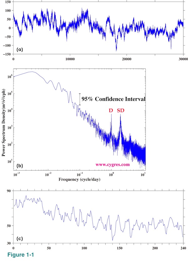
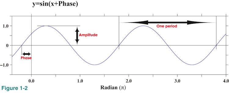
We adopted a widely used method to compute PSD. This method decomposes input data into a series of sinusoidal curves of different frequencies and then evaluates their amplitudes. Figure 1-2 shows a shape of a sinusoidal curve. If a time series plot of data shows sharp corners, sudden jumps, spikes and/or step-like shapes, PSD of that data might show somewhat confusing results. For more about PSD please click ->here<-. We designed this package deal service for customers who wish to take a quick look at a PSD of their data without spending too much time to determine the proper computational parameters shown in Table 1 below. It is usually very difficult to know the best choices of these computational parameters without actually computing and checking the result first. Therefore, we provide results of 9 different PSD computations for a single order of PD001A. (PD001B contains only one result.)
In this document we describe a summary of this package deal service including price information in section (1). In section (2) we describe products (outputs) of this package deal service and possible applications of them. In section (3) we describe how to prepare data for this package deal service using Microsoft Excel. In section (4) we provide some information to help our customer choose adjustable parameters. We use words "frequency" and "period" interchangeably in this document. The relationship between them is that period is inverse of frequency; period=1/frequency (for example, period of 2 cycle/second variation is 1/2=0.5second). Higher frequency is equivalent to shorter period and lower frequency is equivalent to longer period. We use words 'time domain' and 'frequency domain'. Figure 1-1(a) is a simple presentation of data in time domain and Figure 1-1(b) is a counterpart of Figure 1-1(a) but in frequency domain. In this document we treat time series data, but if your data is a one dimensional space distribution of something such as brightness of a material scanned by a moving optical sensor, please interpret the word "time" as "space".
In this document we tried to avoid using technical terms and mathematical equations as much as possible to accommodate wide range of our cutomers. We do not describe the detail of theoretical basis of PSD computation. Instead, we focus our attention on the practical aspects of PSD computations such as how the results of actual computations look like, accuracies of actual computations and such. Certain expressions we use are not mathematically and/or statistically precise.
(1) Summary of PD001A/B
(1-1) What this Package Deal service, PD001A does
A summary of PD001A is shown in Table 1A below. Please note that we compute phase only for Case A1 and amplitude spectrum for Case A1, Case B1 and Case C1 because those values are not useful for other cases as we will describe later. We will provide all of these results (9 cases) for a single order. The reason why we compute all of these cases is that it is usually difficult to know appropriate computational parameters without computing and seeing the results first.
Detrend is the procedure of removing a straight-line least square approximation of data from data and we will describe about detrending in (4-1). For the percentage of confidence interval of PSD, please see (2-1-2-4) and (2-1-3-2). The bin-width of Frequency Domain Smoothing (FDS for abbreviation) is the width (number of bin) of the un-weighted moving average we explicitly apply to PSD. This procedure is very much like the application of simple moving average to time series data to smooth a jagged line. For more detail, please see (4-3). Our customer can specify two different bin-widths for each window function but they must be odd integers (such as 3,5,7,9,11...). If our customer does not specify bin-widths, we will apply default values shown in Table 1. Here, we would like to mention that these default values might be too small to be useful if number of data is large.
Since a Hanning window function has an implicit effect similar to 3 points weighted moving average, actual smoothing bin-width, shown as numbers in parenthesis, becomes wider than explicit smoothing bin-width (number our customer can specify) when a Hanning window function is applied. Similar implicit FDS may occur if our customer chose large taper ratio for a Tukey window function. If our customer select a default taper ratio the effect of an implicit FDS is very small. We describe how taper ratio affects characteristic of a Tukey window function in (4-2-10).
We compute PSD and other variables at frequencies between 0 and 1/(Sampling interval multiplied by 2). Here, sampling interval is time duration between consecutive data point. The frequency interval of these values is constant and equal to 1/(Number of data multiplied by sampling interval)=1/Data length. Please, note that data length is NOT a number of data. For example if sampling interval is 5 seconds and number of data is 200, your data length is 5x200=1000 seconds, the maximum frequency is 1/(5x2)=1/10=0.1 cycle/second (or Hz), frequency interval is 1/1000=0.001 cycle/second and the number of frequencies where PSD and other variables are computed is (0.1-0)/0.001+1=101 (The last +1 comes from the fact that we compute value at 0 frequency as well).
(1-2) What PD001B does
A summary of PD001B is shown in Table 1B. We will provide only one case for PD001B and we do NOT provide graphs. We do not compute amplitude spectrum and phase if FDS is applied because those values are not useful as we will describe later. Also, we do not compute phase if a window function is applied for the same reason. Table 1C shows the difference between PD001A and PD001B.
(1-3) Summary of selectable computational parameters
Our customers can specify following computational parameters individually except for confidence interval percentage ((1-3-2)).
(1-3-1) Detrending data (Applicable to all cases)
Selection is 'yes' or 'no'. Default is 'yes'. In some special cases, detrending data might cause problems as we will describe in (4-1-3). For more detail, please see (4-1).
(1-3-2) Confidence interval percentage (Applicable to all cases)
Default is 95%. Typically used percentages are 80, 85, 90, 95, 99 and 99.5%. We do not recommend choosing any other percentages. It probably does not make sense to change this value for individual case. Therefore, same confidence interval percentage will be applied to all the cases. For more detail, please see (2-1-2-4).
(1-3-3) Taper ratio of Tukey window (Applicable to cases B1, B2 and B3 of PD001A. Also applicable to PD001B if Tukey window is selected.)
Default is 10%. Any value between 0 and 100% is possible although 0% taper ratio is equivalent to no-window (PD001A: cases A1~A3) and 100% taper ratio is equivalent to Hanning window (PD001A: cases C1~C3) and, thus, we do not recommend selecting 0 or 100%. For more detail, please see (4-2) (or (4-2-10) if you know what window functions do).
(1-3-4) FDS bin-width (Applicable to all cases except for cases A1, B1 and C1 of PD001A. Also applicable to PD001B.)
Our customers can chose two FDS bin-width settings for each window function for PD001A. Defaults are 3 and 7. For PD001B our customer can chose one FDS bin-width and the default is 3. Values must be positive odd integers and must be less than half of number of data. Choosing 1 is equivalent to not applying FDS at all. For more detail, please see (4-3).
(1-4) Computational procedure
We take several steps to compute PSD. We first remove a linear trend from data using a least square method (detrending) if it is required. Then we apply a window function if it is required. After that we compute PSD and amplitude spectrum. Next, we correct results if we applied a window function. Then we smooth PSD by applying a moving average (FDS) if it is required. As a final step, we compute percent of variance. The PSD we provide is one-sided PSD (For about one-sided PSD, please see (2-1-2-3)).
(1-5) Your Data (Input data)
Data file must be an ordinary English ASCII coded text file (usually called as a text file) containing only numbers separated by a comma (Excel CSV file) or a space between them. Please note that we do not handle non-English two-byte ASCII coded files. Numbers can be either in an ordinary notation such as -123.4 or in an exponential notation such as -1.234E2, -1.234E02 and -1.234E+2 (Values of all of these are the same). To create a data file for this package deal service from a typical Excel file, please see section (3). Other requirement is that the sampling interval must be constant. If sampling interval of your data is not constant, we could generate constant sampling interval data by interpolation, but that will cost extra. If number of data is not even, we will add one zero value data to make it even for free. This procedure is known as zero padding.
Please note that we will not check the validity of your data for this package deal service. For example, even if all of the values in your data file are exactly zero, we will still compute PSD. For that reason we strongly recommend that you check your data by making a simple time series plot similar to Figure 1-1(a) and inspecting it visually before sending us your data file. In case your data contains some erroneous values, we could treat erroneous values as missing data and fill in the gaps by interpolation for an additional cost. If you can specify interpolation method, data to be interpolated and we do not need to check the result of interpolation, then the additional cost could be as low as only a few US dollars. If your data is a binary file or an ASCII text file but of a complicated format, we still might be able to process your data by writing a program. However, procedure like that might cost a lot (more than few hundred US dollars). Please contact us before ordering this package deal service if sampling interval of your data is not constant, your data contains erroneous values and/or your data file is not a simple ASCII text file. We will estimate the additional cost for free.
If you provide us unit of your data and sampling interval, we will use that information in graphs. Otherwise, all the labels of graphs will not have any unit. In case of Figure 1-1(b), unit of data is meter/second and the unit of sampling interval is hour.
(1-6) Products
We will provide graphs and data files containing PSD and other variables for PD001A. For PD001B we do NOT provide graphs. Summary of products is shown in Table 1A and Table 1B.
(1-6-1) Data file (Product file)
We call data file we provide a product file to avoid confusion between our (output) file and your (input) file. Product files are ordinary English ASCII coded text files and they contain only numbers and commas except for the first line. The first line is a header line and it explains content of each column. Detail of the content is described in section (2). For your convenience we will add a file extension ".csv" so that double clicking our product file will start Excel and read it automatically if Excel is installed on your computer. You can also read our product files using almost any text editor. We use Windows standard line break (carriage return) code for these files. Line break codes for Linux, Windows and older Mac are all different but majority of applications today can handle any type of line break code (example of the exceptions is Notepad of Microsoft).
(1-6-2) Graphs (Figures) in PDF (PD001A only)
We will provide graphs of PSD in PDF format for PD001A. We do not provide graphs of any other variables such as amplitude spectrum.
(1-7) Price and ordering procedure
PD001A computes PSD and amplitude spectrum of one data set (variable) for 20.0 U.S. dollars, which includes PayPal transaction fee. The number of data in a data set could be up to a few million. If you have more than one data set, we will process them for 10.0 U.S. dollars per one additional data set. We do not apply this discount if orders are separated. Price of PD001B for one data set is 10.0 U.S. dollars, which includes PayPal transaction fee. If you have more than one data set, extra cost is 5.0 U.S. dollars per one additional data set for PD001B.
The ordering procedure is as follows;
Step (1) Send us an email to notify us that you are intended to place an order.
Please notify us how many data sets you want us to process and make sure you are interested in ordering PD001A or PD001B. We check our schedule and reply to you how long it would take to process your data as soon as possible. For our email address, please click ->here<-
Step (2) If our schedule is acceptable send us another email with your data.
We will send an acknowledgement and will start processing your data.
Step (3) Once we finish processing your data, we send you a graph in jpeg format as a proof of work.
The graph we will send is a PSD of Case A1 (no-window, no FDS) for PD001A and will have our URL printed on it. If you order PD001B the graph of PSD we will send covers only the lower half of entire frequency range.
Step (4) Please inspect the graphs.
After the confirmation, please, make a payment via PayPal. Please click ->here<- for the payment.
Step (5) As a final step
Once we confirm your payment, we will send you product file(s) and graphs in PDF format via e-mail.
Please note that we do NOT keep your files as described below.
(1-8) Confidentiality
We do not reveal our customers' information and their data to any third party except in the case when we are ORDERED to submit information by Japanese courts or law enforcement offices. We will delete your data and our product files approximately one week after the completion of the work. As for the record keeping, we will keep your mail address, date of work and a control file which controls the program of this package deal service. The control file does not contain any value of your data.
(2-1) Product files
Product files are ordinary English ASCII coded text files. The format of all of these files is the same and they contain variables shown in Table 2A for PD001A and in Table 2B for PD001B.
(2-1-1) Format of Product file
The first line of the product file is the "header" line and this line shows the content of each column. Below this header line there are (Number of data/2)+1 rows (lines) and each row contains the result for a single frequency. Contents of these rows are shown in Table 2A and Table 2B. We will describe detail of these contents in the next subsection. All the numbers are in exponential notation (-1.234E2 instead of -123.4) and we use comma to separate numbers (CSV format for Excel).
(2-1-2) Explanation of contents of product files
(2-1-2-1) Frequency
PSD and other variables are computed at frequencies ranging from 0 to 1/(2 x Sampling interval) with constant interval. The number of these frequencies is (Number of data/2)+1. The interval of the frequency, or frequency resolution, is equal to the inverse of the data length, 1/Data length=1/(Number of data x Sampling interval). For example if sampling interval is 5 seconds and number of data is 200, the minimum frequency is zero and the maximum frequency is 1/(2x5)=1/10=0.1 cycle/second (or Hz), the number of frequencies where PSD and other variables are computed is (200/2)+1=100+1=101 and the frequency interval (resolution) is 1/(200x5)=1/1000=0.001 cycle/second (Hz).
It is important to note that we cannot choose arbitrary frequencies. Data length and sampling interval automatically determine all the frequencies where PSD and other variables are computed. The frequencies we write in product files are these frequencies. One could consider PSD we compute is PSD of bins, centers of those are the frequencies described here. The frequency bandwidth of these bins is constant and equal to a frequency resolution. In other words, frequency coverage of a specific bin is from central frequency (as written in our product file) of that bin minus half of a frequency resolution to central frequency of that bin plus half of a frequency resolution. Using above example, frequency bandwidth=frequency resolution=0.001 cycle/second for all the bins. For the third bin, the central frequency is 0+((3-1)xfrequency interval)=2x0.001=0.002 cycle/second, the lower frequency limit is central frequency-(frequency bandwidth/2)=0.002-(0.001/2)=0.002-0.0005=0.0015 cycle/second and the upper frequency limit is central frequency+(frequency bandwidth/2)=0.002+(0.001/2)=0.002+0.0005=0.0025 cycle/second. We use this concept of bin frequently in this document. We would like to make a note that PSD and amplitude we write in our product file are the values computed at central frequencies of each bin but they are not average values within each bin.
The unit of sampling interval determines the unit of frequency. For example, if our customer tells us that sampling interval is 4ms, the unit of frequency will be cycle/ms. We do not convert unit unless our customer requests it specifically.
(2-1-2-2) Period
Period is equal to inverse of frequency (1/Frequency). Actual period of the first bin (second line of the product file) is infinite because frequency is zero. We write -999.9 for the first bin to avoid possible problem when our customer try to import our product files into other applications for further analysis. Except for the first bin, period is always positive. Unit of period is the same as the unit of sampling interval. The reason why we include redundant information, both frequency and period, is that we thought that it will be convenient for our customers.
(2-1-2-3) PSD
PSD is either defined as two-sided (double-sided) or one-sided (single-sided) PSD. Both of these definitions are widely used. The two-sided PSD is defined both at positive and at negative frequencies, but the values are symmetrical with respect to the zero frequency. For example PSD at frequency -f is the same as PSD at frequency +f. On the other hand, one-sided PSD is defined only at positive frequencies and the value of one-sided PSD is equal to two-sided PSD at positive frequencies multiplied by two except at zero and at highest frequencies. What we write in our product file is this one-sided PSD since we cannot think of any practical advantage of choosing two-sided PSD and we do not lose any information by choosing one-sided PSD.
In the case when we apply a window function we correct PSD. We will describe detail of this correction in Section (4-2-8). Unit of PSD is square of the unit of input data divided by unit of frequency.
(2-1-2-4) Confidence interval of PSD
We compute confidence interval of PSD using commonly used equations. Basic idea is similar (but not equal) to that of the confidence interval of average we described ->here<-. For the detail about how to use confidence interval, please see (2-1-3-2).
(2-1-2-5) Percent of variance
First of all, variance is the statistical quantity, which is often considered to be related to "power" or "energy" of variations. If we detrend original time series data, variance of detrended data is the average of the square of detrended data and this is where the relation between this statistical quantity and the concept of power or energy comes from. Kinetic energy of a moving car is the square of speed multiplied by a mass of that car and divided by two and electric power consumed by a motor is the square of current run through that motor multiplied by the resistance of that motor; both of them are proportional to the square of something.
PSD of a specific bin multiplied by frequency bandwidth is equal to the variance included in that bin and the summation of variance of all of the bins except zero frequency bin is equal to the variance of time series itself. Here we assumed that the average is removed from time series. This can be expressed as, using the fact that the bandwidth is a constant,
From above, the ratio of PSD of a specific bin multiplied by frequency bandwidth to the variance of time series shows how much of total energy is included in that specific bin. This is what we call 'Percent of variance'.
![]()
Please note that PSD of the first bin (m=0) is PSD of zero frequency (time invariant term) and excluded from equation (1) because it is not related to the variations of data at all. If data is not detrended PSD of zero frequency is square of average of data multiplied by data length. If data is detrended PSD of zero frequency becomes zero.
Another thing to be noted here is that the frequency coverage of the highest frequency bin is from the frequency of that bin minus half of a frequency resolution to the frequency of that bin. This means that the bandwidth of the highest frequency bin is half of those of others. This is because PSDs at frequencies beyond of the highest frequency are actually PSDs at negative frequencies. For this reason, we do not multiply PSDN/2 by two when we compute PSD as we described in (2-1-2-3).
(2-1-2-6) Amplitude (Amplitude spectrum)
The time series data, to which we compute PSD, can be expressed as sum of sinusoidal functions of frequencies described in (2-1-2-1). The amplitude spectrum is the amplitude of these sinusoidal functions. Using an equation,
Amplitude spectrum is the value Am in equation (3). This amplitude is a half of peak-to-peak amplitude as shown in Figure 1-2. Please note that Am does not change in time. This fact becomes important later. Our customer can use this variable to estimate amplitude of variation at a specific frequency. We correct values of amplitude when we apply a window function. This correction is slightly different from the correction applied to PSD and we will describe detail of this in section (4-2-8). Unit of amplitude is the same as the unit of data. Amplitude spectrum becomes the square root of PSD multiplied by bandwidth and 2 if a window function is not applied. When a window function is applied this relationship does not hold due to the difference of correction. We will describe more about amplitude spectrum in (2-1-3-3). We do not provide this information for the cases when we applied FDS because FDS would produce meaningless result for amplitude spectrum. We will describe this issue in (4-3-2).
(2-1-2-7) Phase
Phase, as shown in Figure 1-2, is Sm in the equation (3). Phase is usually ignored when we compute PSD but it is not necessarily useless. As equation (3) suggests, one could calculate filtered time series by using only Am and Sm of interested frequency range. This will be explained more in (2-1-3-5). Because we cannot think of any other usage of this information, we only provide this information in the case when we do not apply any window function and FDS (Table 1A; Case A1, Table 1B). The filtering method we describe in (2-1-3-5) only reproduces distorted time series data if we apply a window function or FDS. Unit of the phase is radian (Pi radian=180 degree).
Next Page
