


This page explains what the EOF is and how the customer can use them. This page describs a part of the data analysis services we offer at CRI. Please click "Data Analysis" button above to see other types of data analysis we offer.
2. Complex time domain EOF
2-1 What is it?
The complex time domain EOF was introduced to analyze a group of time series data sets that have coherent variations with phase lag among them. We would not get into any further detail of mathematics but show an example of this type of EOF right away.
2-2 Example
The data sets we use here are the same as those we used before (Figure 1a). Figure 6a shows time series plots of mode 1 and mode 2 components at 40m. We multiplied mode 2 component by 3.0.
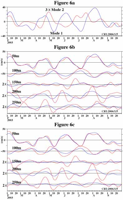
Since phase lag of coherent variations among time series data sets is now allowed, not only the amplitudes but also the shapes of these components vary at different depths. Figure 6b shows mode 1 component (blue line) and input data (red line, same as blue line in Figure 1a) at several depths. Those at depths below 150m are multiplied by 2.0 because their amplitudes are too small to see without magnification.
For the comparison, we made a similar figure, Figure 6c, for non-complex time domain EOF described in section 1-2. In this case only the amplitudes and signs ("hills" becomes "valleys" or the other way around; sign is actually a part of amplitude) of time series data sets generated by EOF vary at different depths but the positions of "hills" and "valleys" do not change. Comparing Figure 6b with 6c, it appears that the time series data sets generated by complex time domain EOF achieved better agreement with input data, especially at 250m.
Figure 6d shows how much of the variations included in the entire original time series data sets (variance) is included in each of EOF components. The mode 1 contains 60.2% of variance of the entire original time series data sets. This is 6.7% higher than the case of non-complex time domain EOF (Figure 2b).
Figure 6e and 6f show how the amplitude and phase of mode 1 vary vertically. Here, the phases at depths other than 40m are relative to the phase at 40m (0.0 at 40m). These are eigenvectors similar to the one shown in Figure 2c (blue line) but eigenvectors of complex time domain EOF are complex numbers. Thus, they have two characteristics, amplitude and phase.
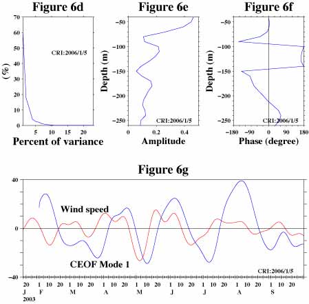
The amplitude (Figure 6e) corresponds to the absolute value (if a value is negative, make it a positive value by changing the sign) of the amplitude shown in Figure 2c. The amplitude of mode 1 is the largest near the surface and it decays rapidly as depth increases to about 80m. It starts increasing as depth increases from there and reaches its maximum at about 120m and then it decays again as depth increases.
The phase at 100m is about +180 degrees. This means that the variations at 100m, where the amplitude is relatively large, are opposite (mirror image) to those at 40m as shown by Figure 6b (blue lines; variations at 50m are shown instead of those at 40m). The phase between 100m and 140m is about +180 degrees but +180 degrees is equal to -180 degrees. Therefore, huge jumps at about 90m and 140m are not really huge at all. Any value which is larger than +180 degrees is shown as -180+value in this figure.
Figure 6b shows that the prominent variations of mode 1 time series (blue line) at 250m are lagging behind those at 200m. Their relationship is not just a simple mirror image. The important point about phase is that we can get this kind of information and this kind of informattion could be very useful to understand how the ocean responds to wind forcing. The non-complex time domain EOF described in section 1-2 allows only 0 and 180 degrees phase differences.
Figure 6g shows time series plots of mode 1 (blue line) and east-west wind speed (red line). The time series plot of mode 1 of non-complex time domain EOF is shown in Figure 3a.
2-3 Some cautions of using complex time domain EOF
We still need some cautions when we use complex time domain EOF.
(1) Variables represented by eigenvectors (phase and amplitude) and eigenvalues are supposed to be constant in time.
This is basically the same as (2) of section 1-3, so we would not repeat explanation.
(2) Complex time domain EOF allows constant phase lag but constant phase lag does not mean constant time lag.
Let assume we have two sets of time series data and all of the variations of one of them lag behind those of others by 30 degrees. In this case we say that there is a constant phase lag between them. However, time lag between them varies depending on period (or freqeuncy) of variation we are interested in. For example, the time lag of variation, period of which is 50 days, between them is about 4.2 days and the time lag of variation, period of which is 100 days, between them is about 8.3 days. The reason why variations of mode 1 time series (blue line) at 200m and 250m look similar except for appearent time lag between them is that the prominent variations of mode 1 are concentrated within relatively narrow period (frequency) range and within that range, diffrence of time lag is relatively small.
If there are certain reasons to believe that coherent variations among time series data sets have constant time lag among them rather than constant phase lag, then using complex time domain EOF might not be a good idea. Applying a band-pass filter before computing complex time domain EOF might reduce the risk of this problem. Alternatively we might try using frequency domain EOF, which will be described later, in the case like that.
3 EOF for vector data(Complex, time domain)
We described a family of EOF applied to time series data sets that have only one variable (scalar data) up to now. We picked up east-west component of oceanic velocity data in our previous examples but velocity data also have north-south component. Since the equator is geophysically rather a special place, picking up only the east-west component of ocean current makes sense. However, we might want to analyze east-west and north-south components simultaneously (vector data). Can we do that? Yes. We can apply EOF to vector time series data sets. We generate complex time series data sets using east-west components as real parts and north-south components as imaginary parts of them. After that we apply EOF to these complex time series data sets just like in our previous example of complex time domain EOF.
We omit examples for this type of EOF here because we do not have any good data to demonstrate usefulness of this method.
4 Frequency domain EOF (complex)
4-1 What is it?
In short, the frequency domain EOF is a principal component analysis applied to a matrix of cross-spectral density function. Roughly speaking the cross-spectral density function shows relationships between two time series data sets at different frequencies. The frequency domain EOF is computed separately at each of these frequencies. Thus, this type of EOF allows different phase lags at different frequencies among input time series data sets unlike complex time domain EOF. This particular feature is quite useful for certain cases.
4-2 Example
We used same data sets as before except that we did not apply a band-pass filter because we can select frequencies where we compute frequency domain EOF without using a band-pass filter. In this example we computed frequency domain EOF at 12 frequency-bands. Figure 7a shows how the square of amplitude of mode 1 variations distributes in the depth-period space. The vertical black solid lines indicate center frequencies of these frequency-bands. We converted values in this figure so that we can compare this figure with power spectral density (PSD) (Figure 7b) which is proportional to the square of amplitude of variations of original data sets at each frequency. In both figures, we show log 10 of results because ranges of values are very wide. The largest value in these figures (dark red) is actually 100000 times larger than the smallest value in these figures (dark blue).
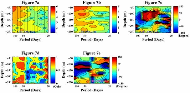
Figure 7b shows that the variations of original time series data are large (red-orange area) at periods longer than 40-day near the surface (upper part) and at periods between 40 and 80-day with maxima at about 110m, 180m and 230m. The amplitude of the maximum near 110m at about 50-day period (dark orange blob) is more than 100 times larger than the amplitude at periods longer than 80-day or at periods shorter than 45-day (green-blue) at that depth. Comparing figure 7b with 7a we can see that the patterns of these two figures are quite similar.
Figure 7c shows phase of mode 1. Phases at depths from about 70 to 100m and at periods from about 80 to 60-day do not jump from one extreme to another. -180 degrees (dark blue) is equal to +180 degrees (dark red). This figure shows that the contour lines at periods longer than about 30-day are mostly horizontal. This means that the vertical variation of phase is relatively independent of period, and it suggests that the applying complex time domain EOF instead of frequency domain EOF to this data set might not be a bad idea.
Figure 7d and 7e show coherency function and phase between mode 1 and east-west component of wind speed, respectively. Figure 7d indicates that the mode 1 of ocean current speed is strongly related (value of coherency function is close to 1.0) to wind speed at periods between 40 and 80-day. Figure 7e indicates that the variations at 40 to 80-day periods between about 100 and 150m are 180 degrees different from (mirror image to) those near the surface and those below 150m as suggested by previous example of complex time domain EOF.
As we have demonstrated here, we can obtain more detailed information about variations from frequency domain EOF.
4-3 The relation between complex time domain EOF and frequency domain EOF
The result of complex time domain EOF becomes practically the same as the result of frequency domain EOF if we applied a band-pass filter (referred to as BPF), which allows narrow frequency range to pass through (referred to as passband), to input time series data sets before computing complex time domain EOF. However, the caveat is that it is not necessarily easy to construct a low distortion (good) narrow passband BPF. Also, if we applied a narrow passband BPF to a time seris data, resultant filtered data looks like simple single frequency sinusoidal variation with slightly varying amplitude. Time series data such as that is not that much suited to compare with others visually because it tends to lose noticeable features to compare with.
We did following computations for a demonstration. First of all, we applied a BPF, passband of which is 121-day to 20.2-day period, to the data sets at depths between 40 and 80m (5 data sets). Then we computed complex time donain EOF using these filtered data sets. For this experiment we have chosen relatively wide passband because it is difficult to construct a good narrow passband BPF.
Separately, we computed freqeuncy domain EOF in the following manner. First of all, we computed cross-spectral density function using same data sets (not filtered). Then we applied freqeucny domain smoothing. We picked up one frequency band which covers 121-day to 20.2-day period (13 bands, same period range for complex time domain EOF) after frequency domain smoothing and computed freqeuncy domain EOF for this band.
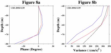
The blue line of Figure 8a shows phase of mode 1 of frequency domain EOF and the red line shows phase of mode 1 of complex time domain EOF. Figure 8b shows variance (proportional to the square of amplitude) of mode 1 of EOFs. The black line in this figure shows variance of original time series data sets for a comparison. The results of these two methods are reasonably close.
4-4 Some cautions of using frequency domain EOF
(1) How to compare the results of frequency domain EOF with other time series data sets that are not included in the computation of frequency domain EOF
If you want to compare results of frequency domain EOF with other time series data sets, we recommend computing a coherency function directly as we did in our example. It is possible to generate new time series data sets using results of frequency domain EOF and then compare them with other time series data sets but we think using time domain EOFs is much more straighforward if what we want to have are new time series data sets.
(2) The nature of variations might be quite different at different frequencies even if they are in the same mode.
This is because we compute frequency domain EOF at each frequencies independently. The vertical black lines in Figure 7a shows these frequencies (periods). The result at any frequency is independent of the results at other frequencies if they are outside of the range of freqeucny domain smoothing. The range of frequency domain smoothing is three in our example (Figure 7) and it means that the result of EOF at any frequency band is related only to the results at one band left (longer period) and one band right (shorter period). So, for example, there is no guarantee that the mode 1 at about 100-day period has any relation with the mode 1 at about 40-day period. It is possible that the responses caused by the same source might become mode 1 at some frequencies but become mode 2 or other modes at other frequencies. Therefore, it needs some cautions to interpret figures like Figure 7a and 7c.
As a matter of fact, you might have noticed that the values of coherency function in Figure 7d sharply decrease at period slightly shorter than 50 days (green-blue area centered at about 40-day period). Figure 9a shows coherency function between east-west component of wind speed and original ocean current time series data without applying EOF. Figure 9b is the copy of Figure 7d; coherency function between east-west component of wind speed and mode1 of frequency domain EOF. Figure 9c is the coherency function between east-west component of wind speed and mode 2 of frequency domain EOF.
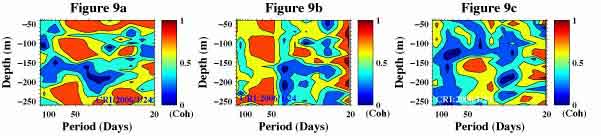
The high coherency function area between mode 1 and wind speed is wider than the high coherency function area between original ocean current and wind speed at periods longer than 40-day (longer period). Figure 9a shows that the ocean current at about 40-day period is still highly coherent with wind speed. Figure 9c suggests that the variations of ocean current highly coherent with wind variations at this period become mode 2 instead of mode 1 at depths below about 140m.
5 Rotary EOF (complex; frequency domain )
In the ocean there are motions that rotate clockwise or counterclockwise. The rotary EOF was used to detect those motions. It uses complex time series data sets, real parts of which are east-west components of velocities and the imaginary parts of which are north-south components of velocities. The next step is computing cross spectral density function matrix of these data analogous to the computation of rotary cross spectral density function. Then we can compute EOF just like ordinary frequency domain EOF. As such, this method is basically for the vector data. We omit examples for this EOF because we do not have any good data to demonstrate usefulness of this method.
please send a mail
-->here<--
Announcement
We started offering low cost micro-job style computational services. For more information, please click >here<.
