


This page explains what the confidence interval for the average is and how the customer can use it. The computations of confidence interval for the average and others described in this page are a part of the data analysis services we offer at CRI. Please click "Data Analysis" button above to see other types of data analysis we offer.
First of all, we use a word "average" throughout this page. The word "mean" is quite often used as a substitute of the word "average" but the word "mean" has several different meanings as this sentence itself shows and, thus, we avoid using the word "mean".
We explain how certain the value of the average is. We also explain how to know if the difference between values of individual data and the average computed from those data is negligible or not and how to know if the difference between averages computed from two groups are negligible or not.
Population and samples
We quite often use words "population" and "sample" in the statistical analysis. Let 's say we want to know the average height of people aged between 20 and 24 years old in your country. Then, the "population" is all the people aged between 20 and 24. It is usually quite difficult to get data from all of these people due to the cost. So, what we usually do is to pick up some of these people and get data from them. The "samples" are these people we picked up. We then compute average from these samples and call the result the average height of people aged between 20 and 24 in your country. What we did here is estimating the average of "population", let us call it "true average" in this page, from "samples" and we made a silent assumption that sample average is the same as true average. Then, skeptical people might ask if that assumption is correct or not. In reality, they are usually not the same. As you might expect, the exact value of sample average would change even if you replace only one of the sample by another in the population. What this means is that the value of sample average has an uncertainty. So, the question is how much that uncertainty is.
Our example; normal distribution
Figure 1a shows frequency distribution of population A we use as an example in this page. This population contains 100000 (0.1 million) data. Before going any further, we would like to introduce "normal distribution" briefly at this point. There are many cases when data of various kinds show so-called normal distribution that is shown as a red bell shaped curve in figure 1a and 1b. There are some other cases we can transform non-normally distributed data into normally distributed data by applying some simple mathematical transformation. Because of this generality, the characteristics of normally distributed data are well studied in the past. Thus, we made our example populations that are randomly but normally distributed. Figure 1b shows frequency distribution of another population named B. This population is also distributed normally.
Announcement
We started offering low cost micro-job style computational services. For more information, please click >here<.
please send a mail
-->here<--
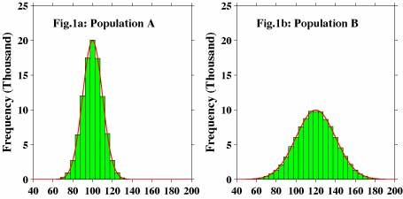
We usually compute standard deviation as a first step to evaluate how certain average is. The standard deviation shows how scattered data are from their average and it becomes larger as the data scatter more. We then compute confidence interval of the average from this standard deviation. At this point, we have to specify how certain this interval is by means of the percentage that is called confidence level. For example, 95% confidence interval means that if we extract samples from the population and compute confidence interval for average of them each time repeatedly (sample average differs each time because samples are not the same), the average of the population would fall in these intervals for the 95% of the time. Thus, we say that the confidence of calculated confidence interval for the average is 95%. In this way we know how certain the average computed from sample as an estimate of true average is. We customary use confidence interval of 99, 95 or 90%.
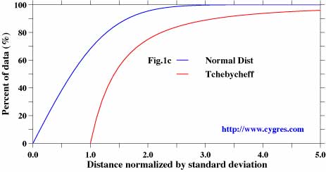
Standard deviation is also useful to know how many data exist within the specific interval from the average as the Tchebycheff's theorem dictates that there are more than 1-1/C^2 (C^2 means square of C, C must be greater than 1!) data within the interval of C times standard deviation from the average. The blue line in figure 1c shows how many data are included within the specific distance, which is measured by standard deviation in this figure, from the average when data are distibuted normally. In this case, there are 68.3% of data within the distance of one standard deviation and 95.5% of data within the distance of the twice of the standard deviation . Tchebycheff's theorem (red line) results smaller values but the good thing about this theorem is that it applicable to non-normally distributed data.
How many samples do we need?
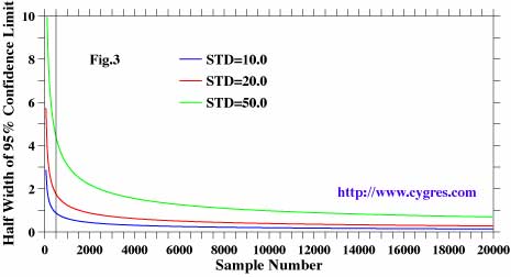
The number of samples you extract from population also affects the confidence interval for the sample average. Figure 3 shows how the half width of the 95% confidence interval for sample average changes as the number of sample changes. The standard deviation is fixed and we computed for three cases. This figure shows that the confidence interval decreases rapidly as the number of sample increases initially. Decrease of confidence interval means you can get more accurate estimate of true average. However, this trend slows down as you extract more samples from population and, eventually, the confidence interval would not decrease that much any more. Your effort to obtain more data will not be rewarded that much at that point. Therefore, you have to have a strategy to know just how many samples you need to have because obtaining data usually costs some money. You have to have three numbers to know how many samples you need. First of all, you have to specify the confidence level. We customary choose 99, 95 or 90% as described before. Next, you have to determine how much possible difference between sample average and true average, the width of confidence interval, you can accept. At this point you basically have determined the certainty/accuracy of sample average you can have. Then, you need to have an estimate of standard deviation of population. You can estimate it based on past experiences or just give a rough estimate. From these three numbers you can draw a figure similar to figure 3 and estimate how many samples you need to accomplish your task. If you are not so sure about your estimate of standard deviation of population, you could repeat computations with the different value of standard deviation of population and make your decision based on those results along with your financial resource. Figure 3 indicates that 500 samples (the vertical black line) were enough for population A but we probably needed more samples for population B in our examples
The value of my data is different from sample average. Is this difference significant?
If the value of your data falls in the confidence interval for the sample average, then your data are not statistically significantly different from the true average because true average is located somewhere in that confidence interval just like your data. However, it is noted that the confidence interval changes if you change the confidence level. Therefore, your conclusion might become opposite if you change confidence level.
The averages of sample A obtained from population A and of sample B obtained from population B are different. Are these two populations different?
There is a statistical theory how the difference of sample average A and sample average B distribute. We use this theory to check if population A and B are different. We do not use confidence interval but we use standard deviations in this computation. We need to specify confidence level, however.
There are two populations, A and B, and I have data that belong to either population A or B. How do I know to which population my data belong?
The basic idea of solving this problem is to see the distances between the value of your data and the true averages of both populations. Then you decide that your data belong to the population the true average of which is closer to your data. The important point here is that these distances are not simple differences between true averages and the value of your data but they must be weighted by standard deviations of each population. The standard deviation is the measure of how scattered data are as described before. In our example, the boundary between population A and B is at 106.67 which is geometrically closer to A (center point is at 110.0). This is because data belong to population A are less scattered and tend to distribute closer to the true average (100.0) than those of population B. This method can be extended to the cases when data contains multiple parameters. For example, we can use this method to separate the result of agricultural experiments based on information such as length, weight, water and nutrient containment. We can also use similar method to classify samples to groups of more than two.
The size of population is very small and I can easily compute the average of population. Then, why should I bother computing confidence interval?
Let assume you are a teacher and you just gave a test to your student of twenty. It is easy to compute average and standard deviation of the score of 20 students. If you consider the result of this single test as a population, then nothing was left to estimate. However, if you consider the possibility that what you have is just one case of many classrooms where teachers give tests of similar academic level to students of similar academic level, then, you might get better estimate of "true average" score of the test by computing confidence interval.
Another example is that let assume you are an owner of a factory and you want to experiment several new methods to improve quality of products. Then you usually produce limited number of products by these new methods to see how they work. It might be very easy to compute average of those test products. However, are those test products supposed to be samples of millions of products you might produce in the future? If that is the case, what you have is a sample average and calculating confidence interval could be very useful to evaluate the effect of new production methods.
How about ratio such as yes/no vote
When your data are more like number of "yes" or "no" votes rather than continuous numbers such as height, we can still evaluate confidence interval. We can also estimate number of samples we need for a specific accuracy.
We separated our services into several categories for the sole purpose of introducing our services in an organized manner. To serve your needs we do combine our services in different categories.