This page explains what the EOF is and how the customer can use them. This page describs a part of the data analysis services we offer at CRI. Please click "Data Analysis" button above to see other types of data analysis we offer.

We prepared explanatory pages with some examples for underlined words in blue. If you want to see those pages, please click underlined words in blue below.

What is EOF analysis?
In short, the EOF (Empirical Orthogonal Function) analysis is a Principal Component Analysis (PCA) applied to a group of time series data. The word "EOF" is probably a jargon used only among oceanographers and atmospheric scientists. We explain it in more detail with some examples below. We usually use EOF analysis to extract coherent variations that are dominant among a group of time series data for further study. In this document we treat time series data, but if your data is a one dimensional spatial variation of something such as brightness of a material scanned by a moving optical sensor (such as a camera), you can apply EOF in that case too. What we need to do is that replacing words related to time with words related to space.

Why should I bother computing EOF?
The advantage of EOF analysis is that we need to analyze a few, usually just one or two, sets of new time series data generated, or should we say extracted, by EOF from a group of original time series data if those original time series data are relatively coherent each other. This is because these few sets of new time series data could include majority of variations included in the original data that might consist of hundreds of time series data sets. We describe this topic in more detail later with some examples but the point here is that EOF might help us reducing our efforts/costs of analyzing huge sets of time series data considerably. If original time series data sets are utterly uncorrelated each other, it is quite possible that the EOF would not be helpful at all. If we are more interested in classifing multiple sets of time series data rather than extracting coherent variations among them, it might be better using methods such as Varimax which is one of the popular methods categorized as Factor analysis but we only describe EOF/PCA analysis in this document.

Type of EOF
There are several variants of EOF analyses applied in the past. Most of them are categorized as the time domain analyses. However, it is possible to apply EOF in the frequency domain. Looking at time series data in the time domain is convenient if you want to know the sequence (or history; which comes first and which comes later) of events. On the other hand, looking at time series data in the frequency domain might be more convenient if you want to know the frequency of events. Typical frequency domain analyses are the spectral and coherency analyses. These analyses are counterparts of time series plot and correlation analysis in the time domain. The unit of frequency is the inverse of the unit of time. The frequency domain EOF is occasionally called complex EOF but it is somewhat confusing because there are other types of EOF that use complex numbers as we will describe below.

1 The EOF; non-complex and for time domain analysis
1-1 What is it?
The simplest EOF analysis is the time domain EOF analysis that is basically the computations of eigenvector and eigenvalue of a covariance or a correlation matrix computed from a group of original time series data. If you are familiar with PCA, you probably have noticed immediately that the computation of EOF is basically the same as that of PCA. This type of EOF does not use complex numbers and is best suited if the coherent variations among original time series data have no time lag among them. If coherent variations among original time series data have constant time lag among them, we need to shift data before computing EOF to cancel time lag. This topic will be described in more detail later.

We can extract coherent variations among a group of original time series data and create a new sets of time series data by using original time series data and eigenvectors. One of the important things about these new sets of time series data is that they are statistically non-correlated each other. In other words, EOF extracts coherent variations in the group of original time series data, and separate them into several mutually uncorrelated components (EOF does not do these in this sequence).

Since these new sets of time series data are uncorrelated each other, it is probably reasonable to assume that each set of new time series data represents different phenomenon. Then, we usually try to study each component individually. The magnitudes of eigenvalues show how important each of these new sets of time series data is.


1-2 Example
Figure 1a shows time series plots of current meter records at several selected depths at 147E on the equator (North of Papua New Guinea). If you are not particularly interested in oceanographic data, you could consider these data as whatever the time series data you are interested in such as sales records at different locations.

The vertical axis scale at the upper left is for the record at 50m and we moved all other records downward to make comparison easier. The zero levels for each record are shown as horizontal black lines. We downloaded these data from NOAA, U.S.A. (http://www.pmel.noaa.gov/tao) and applied a band-pass filter to remove variations of period longer than 150 days and shorter than 20 days.

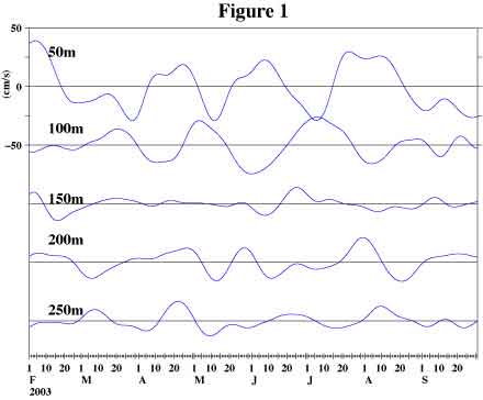
This figure suggests that the variations of current at 100m (2nd line from top) are inversely correlated with those at 50m (1st line) while those at 200m (4th line)might be inversely correlated with those at 100m. There are 23 sets (depths) of time series data at this location if we ignore bad data. Studying the relations among these 23 sets of time series data like this way is an overwhelming task to us.

So, we applied EOF to extract coherent variations among these 23 data sets. Figure 2a shows time series plots of two major components extracted from original time series data. Let us call these components mode 1 (blue line) and mode 2 (red line) following oceanographic tradition. Although it looks like they are somewhat correlated, the correlation coefficient between these two time series data is actually zero (yes, we actually computed).

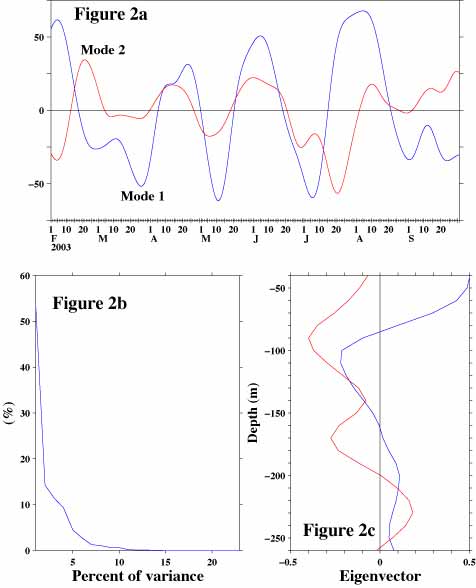
Figure 2b shows how much of the variations included in the entire original time series data sets(all 23 of them) is included in each of these components. For this purpose we used statistical quantity called variance which is often considered to be related to "power" or "energy" of variations. The vertical axis of this figure is the percent of variance and the horizontal axis is the mode number (there are 23 modes). The mode 1 contains 53.5% and the mode 2 contains 14.3% of variance exists in the entire original time series data sets. This information is what we can obtain from the eigenvalues. The variance contained in each mode decreases progressively as the mode number increases. Thus, we can concentrate our analysis efforts on a few lower modes. Even if we ignore many other higher modes we would not lose that much information.

In this case if we analyzed mode 1 and mode 2, then we have practically analyzed 67.8% of variations included in the original 23 sets of time series data. Our efforts/costs to analyze just only two sets of time series data would be considerably lower than our efforts/costs to analyze original 23 sets of time series data. This is why EOF is a useful tool.

Figure 2c, the eigenvectors of mode 1 and mode 2, shows how the amplitude of variations shown in Figure 2a varies at different depths. The mode 1 is positive at 50m, negative at 100m and positive at 200m. This means that the variations at 100m look like mirror images of those at 50m and at 200m except that their amplitudes are different. This pattern matches our previous description of Figure 1.

Other than these qualitative observation, we now know how the amplitude of variation shown in Figure 2a varies at different depths quantitatively. The information like this might help us to identify the cause of these variations. Even if we do not need to know the cause of these variations, knowing the amplitude of variations at different depths quantitatively rather than qualitatively would be probably nice.

So, what is the mode 1 anyway, which includes 53.5% of variance included in the original time series data? Figure 3a shows time series plot of mode 1 (blue line) and east-west wind speed (red line) at 147.5E on the equator obtained from NOAA, U.S.A. (http://www.cdc.noaa.gov/cdc/reanalysis).

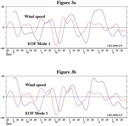
This figure suggests that mode 1 variations of ocean current at this location are related to the wind speed variations. The variations of ocean current lag behind those of wind. The value of the correlation coefficient reaches its maximum, 0.68, when we shift wind data to the right by 9 days. We computed 95% confidence interval assuming that effective sampling interval is 10 days since the cut-off period of a band-pass filter we applied is 20 days, and this correlation is statistically significant (meaningful).

From figure 2c wind influence is such that the ocean current near the surface and at depths below 160m is accelerated in the down-wind direction but it is accelerated against wind direction at depths between about 80 and 160m.

We will stop our analysis at this point since this is not a scientific paper, but we would like to mention that we published results of more detailed analysis applied to the older data at the same location in a scientific journal.

1-3 Some cautions of using EOF
The EOF is just one of the numerical computations based on statistical theories but it is not a magic wand which would automatically extract useful information from a group of complicated time series data. User should pay some attentions to the limitations of EOF.

(1) This type of EOF cannot deal with phase or time lag among time series data sets.
To demonstrate this point we create new groups of data sets consisting of 5 sets of time series data. The first experiment is the case that all of the time series data sets are identical. Theoretically, mode 1 contains all the variations in this case and the eigenvalues of all of the modes except for mode 1 are zero. Our computation shows that the sum of eigenvalues of mode 2 through mode 5 is 0.00000000000000013. This value is not zero but negligibly small. We usually have some numerical errors when we do numerical computations.

Figure 4a shows the data sets for the second experiment. The first time series data (top) is the one at 50m. The second time series data is the same as the first one except that we shifted it backward (to the right on a time series plot) by 5-days. We shifted the third one by another 5-days, totally 10-days. We generated the fourth and the fifth time series data in a similar manner.

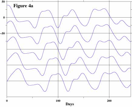
Figure 4b shows time series plots of mode 1 (blue line) and mode 2 (red line). Figure 4c shows eigenvalues of this experiment. Mode 1 contains only about 60% and mode 2 contains about 34% of variance of the input data sets. This result indicates that mode 2 is no longer negligible.

Figure 4d shows eigenvectors of mode 1 and mode 2. Mode 1 has amplitude variations at different "depths" (not a straight vertical line) although all the time series data are exactly the same except for the time shift among them.

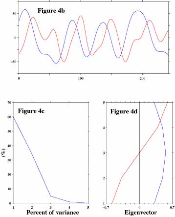
You might have noticed that the time series plots of mode 1 and mode 2 (Figure 4b) look suspiciously similar. The correlation coefficient between them is zero but it becomes 0.81 if we shift mode 2 time series data to the left by 13.3. The zero-correlation among time series data sets generated by EOF is guaranteed only if we do not shift resultant time series data at all.

To avoid result like this we have to adjust data sets before computing EOF if the variations in oroginal time series data sets have time lag among them. Alternatively we might use time domain complex EOF or frequency domain EOF if we do not know how much we need to shift data. We will describe these methods later in this page.

(2) Variables represented by eigenvectors and eigenvalues are supposed to be constant in time
The EOF produces only one set of eigenvalues (Figure 2b) and eigenvectors (Figure 2c). If actual variables represented by these are not constant in time, then the result of EOF might become hard to interpret or, at worst, meaningless. Actually there is a good physical reason to believe that the actual variables represented by eigenvectors would vary in time in our example.

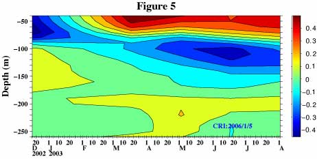
Then, what we can do to deal with this kind of problem is creating a time series of eigenvectors in the following manner. First, we picked up initial 91.25-day (1/4-year) long segment of data and then applied EOF to that segment of data. Next, we picked up another 91.25-day long segment of data starting from 91.25/2=45.625 day (0 day is the start date of entire data) and then applied EOF to this new segment of data. We repeated this procedure until we reached the end of the data. Figure 5, the result of these computations, shows how the eigenvector of mode 1 changes in time. This figure shows that mode 1 eigenvector has a two-layer structure (negative near the surface and positive below) at the beginning of the data. Then, it changes to a three-layer structure (positive near the surface, negative below to about 180m and positive again below) in the early 2003 and this three-layer structure continues to exist till the end of data. Thus, in our example (Figure 2 and 3), we picked up data starting from February 2003 but discarded data prior to that month.

(3) We might need to do some pre-processings before computing EOF
In some cases modifying our data before computing EOF might give us more useful results. One of the example is shifting data as we described above. However, It is very important to remind ourselves that whatever we do to our data before computing EOF, there should be good reasons to do that and we should be able to explain why we do that. Arbitraly preprocessing just to get "prettier" results is not recommended.

In case of our example we know that there are strong tidal signals in our data. We know also that there are variations of periods of half a year and one year. We are not interested in these variations. Also, we have an idea at which frequencies wind has strong influences on ocean currents through coherency analysis. Thus, we applied a band-pass filter to our data before computing EOF based on this prior knowledge. We used a combination of classical numerical filters called Butterworth filter but there are many other numerical filters. It is also possible to use more modern methods such as wavelet analysis.

Another important point here is that a specific external factor might have influences to our data by several different mechanisms via different routes. The responses caused by the same external factor but by different mechanisms might have different characteristics. For example, certain mechanisms might dump variations of shorter period while others might dump variations of longer period. It might become difficult to interpret time series data sets produced by EOF as a result of that. Wind affects ocean currents on the equator in several different ways in our example. We have a theoretical reason to believe that the mechanisms by which wind affects to ocean current near the surface where eigenvector is positive and to ocean current at mid-depths where eigenvector is negative are different. One of the methods we can try in case like this is removing some data sets before computing EOF. So, we re-calculate EOF using data at depths only between 40m and 80m (5 time series data sets). Here, we might say we "filtered" our data based on depth (location). Figure 3b, the result of this re-calculation, shows shorter period variations such as "dual-bump" features more clearly than Figure 3a does.

If we mix time series data sets with different units (units of speed, temperature and such), we usually need to adjust their amplitude unless we use a correlation matrix to compute EOF. This process is called weighting and multiplying certain constant to each of these time series data sets often does it. We usually remove average and often remove trend from each time series data set before computing EOF. Using a correlation matrix to compute EOF is equivalent to adjusting amplitude of input data by dividing input data by the square root of variance of them before computing EOF. By doing so all the time series data sets will have equal importance (weight) in EOF computation.

Finally, EOF might not be able to separate variations caused by different factors especially when they are correlated for whatever the reasons. In case of ocean we have daily variations caused by tidal motions. We have another daily variation caused by solar heating during the daytime and radiation cooling during the nighttime near the surface. Periods of these variations are not exactly the same but it is quite possible that we cannot separate effects caused by these two factors by EOF.

(4) The result of EOF might be meaningless.
Let us generate random numbers and create time series data set using them. These data sets contain no meaning by definition. However, if we apply EOF to these data sets, it still gives us eigenvalues, eigenvectors and time series data set but they are just as much meaningless as input data are. While this is rather an extreme example, there is no guarantee that EOF would extract any useful information in general. There may be the case when we cannot relate the time series data generated by EOF to any known variations. In our previous example EOF gives us 23 components but it is highly doubtful if variations of mode 3 and higher carry any interpretable/useful information. If we are interested in extracting rather weak variations, it would be better if we amplify them (or dump others) by applying appropriate filters and remove unnecessary time series data sets from our data set before computing EOF.

Announcement
We started offering low cost micro-job style computational services. For more information, please click >here<.