


This page explains what the power spectral density function is and how the customer can use it. This page describs a part of the data analysis services we offer at CRI. Please click "Data Analysis" button above to see other types of data analysis we offer.
We prepared explanatory pages with some examples for underlined words in blue. If you want to see those pages, please click underlined words in blue below.
We offer low cost power spectrum density computational services.
For more information please click >here<.
What is power spectral density function?
Power spectral density function (PSD) shows the strength of the variations(energy) as a function of frequency. In other words, it shows at which frequencies variations are strong and at which frequencies variations are weak. The unit of PSD is energy (variance) per frequency(width) and you can obtain energy within a specific frequency range by integrating PSD within that frequency range.
What can you do with power spectral density function?
PSD is a very useful tool if you want to know frequencies and amplitudes of oscillatory signals in your time series data. For example, let assume you are operating a factory with many machines and some of them have motors inside. You detect unwanted vibrations from somewhere. You might be able to get a clue to locate offending machines by looking at PSD which would give you frequencies of vibrations. PSD is still useful even if data do not contain any purely oscillatory signals. For example, if you have sales data from an ice-cream parlor, you can get rough estimate of summer sales peak by looking at PSD of your data. We quite often compute and plot PSD to get a "feel" of data at an early stage of time series analysis. Looking at PSD is like looking at simple time series plot except that we look at time series as a function of frequency instead of a function of time. Frequency is a transformation of time and looking at variations in frequency domain is just another way to look at variations of time series data. PSD tells us at which frequency ranges variations are strong and that might be quite useful for further analysis.
What does power spectral density function of actual data look like?
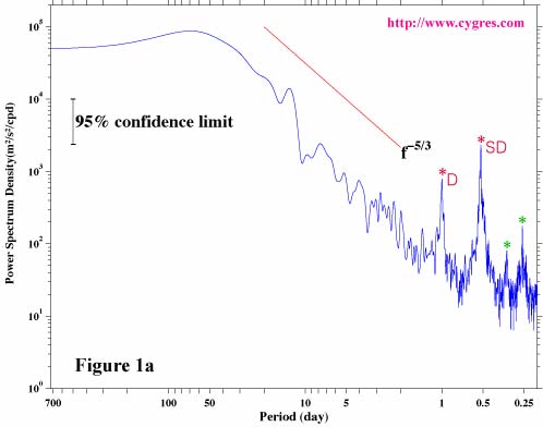
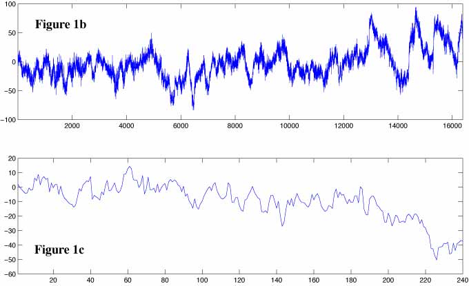
We picked up oceanographic data as an example. Figure 1a shows power spectral density function of east-west(zonal) current on the equator. Data were obtained from the web site of National Oceanic and Atmospheric Administration, U.S.A. (http://www.pmel.noaa.gov/tao). The horizontal axis of this figure is the period. In case of oceanographic data the variations of fixed frequencies such as tides would appear as distinctive sharp peaks. Other than these sharp peaks oceanographic data generally show broad peak, or one might call a hill, at low frequency (long period) range. Energies are fed to the ocean usually from the atmospheric variations at these low frequencies. The energy decreases exponentially from there toward higher frequencies. The energy at these frequencies is transferred from lower frequencies by so called non-linear processes and it will be eventually lost as heat by viscosity at much higher frequencies (shorter periods). The tidal components in Figure 1a appear as sharp peaks at about 1.0 and 0.5-day as well as at 0.33 and 0.21-day. The former two are diurnal (once a day; marked by *D) and semi-diurnal (twice a day; marked by *SD) tides and further analysis indicates they consist of several components of slightly different periods. Later two components (marked by green *)are probably real but they are not so commonly seen. PSD is almost proportional to -5/3 power of frequency at periods from about 50 to 1-day. Figure 1b shows time series plot of input data and Figure 1c shows initial 240 data corresponding to 10 days duration. There supposed to be 10 diurnal cycles and 20 semi-diurnal cycles but those variations are not easy to see without proper filtering although PSD clearly shows the existences of those variations. Thus, this example demonstrates usefulness of PSD.
please send a mail
-->here<--
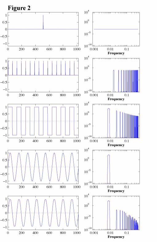
Graphs of PSD such as Figure 1a quite often give us useful information but we need some cautions to interpret them in certain cases. The left panels of Figure 2 show plots of five different sets of time series data and the right panels of Figure 2 show PSD of those. The thin horizontal lines in the left panels indicate zero level.
The single pulse (top row) in the middle of the time series, although its location is unimportant, results flat PSD across the entire frequency range. This is what the theory says. If your data have a strong spike-like noise somewhere, that spike might boost energy level everywhere and make everything else obscure.
The periodic spike signal (second row) produces multiple peaks, called harmonics, on PSD although actual frequency of occurrence of spikes is not multiple but one specific frequency. You might have this kind of data when your data are contaminated by sparks caused by some kind of rotational machinery such as a motor.
If your data have a shape of rectangular wave (third row), you will get harmonics again on PSD. You might encounter a pattern like this if you measure clock outputs of logic circuits. Is this a problem? If you want to know the frequency of rectangular waves as rectangular waves instead of summations of sinusoidal waves, probably yes. However, if you want to know how much bandwidth is necessary for your digital data transmission, the answer might be no. The pattern of digital data is usually not as regular as the example we show here.
All of these confusing results occur from the fact that PSD is basically trying to decompose input data into a series of sinusoidal waves (4th row is a case of sinusoidal wave) of different frequencies. It requires many high frequency sinusoidal waves to reproduce input data properly when input data have signals that have shapes nowhere close to a sinusoidal wave, especially when they have sharp corners.
If input data have a shape of a pure sinusoidal wave (4th row), PSD shows its frequency nicely. The peak of PSD in this figure is not a single point sharp peak (usually called line spectrum) but it has a width of three frequency points. This is because we applied a "spectral window" (we called FDS here) which is necessary to evaluate confidence interval of amplitude but it makes peaks broader. There is a trade off between the accuracies of the estimation of amplitude and of frequency. "Raw spectral"(the result before applying a spectral window) shows a peak at one frequency (band) in this case.
Next, we cut off peaks of this sinusoidal wave so that it has flat tops with sharp corners as a final example (5th row). The amplitude of the signal shown in the 4-th row is 1.0. We clipped values above 0.95 and below -0.95. Situation like this might occur when you have a beautiful sinusoidal wave as an input to your amplifier but the amplitude of the input is too large for your amplifier. Casual look of a time series plot might miss this saturation but PSD would probably remind you about it.
The computational method we used here is the most commonly used method for PSD computation and the examples we showed above are the best possible results. When we need to deal with real world data, we might encounter certain problems such as the phenomenon called spectral leakage. If you need further information about PSD, Section 2, Section 4 and Appendices of our PD001A/B User Guide might be helpful.
What is cross spectral density function?
When we have two sets of time series data at hand and we want to know the relationships between them, we compute coherency function and some other functions computed from cross spectral density function (CSD) of two time series data and power spectral density functions of both time series data. If we have more than two sets of time series data, we might compute frequency domain complex empirical orthogonal functions from cross spectral density function to know the relationships among those data. The cross spectral density function is a Fourier transform of cross correlation function but we can compute CSD directly using a method called FFT.
We offer low cost power spectrum density computational services.
For more information, please click >here<.