Page 7 of PD001A/B User Guide

Table of Content
(1) Summary of PD001A/B
(1-1) What this Package Deal service, PD001A does
(1-2) What PD001B does
(1-3) Summary of selectable computational parameters
(1-3-1) Detrending data (Applicable to all cases)
(1-3-2) Confidence interval percentage (Applicable to all cases)
(1-3-3) Taper ratio of a Tukey window (Applicable to cases B1, B2 and B3 only)
(1-3-4) FDS bin-width (Applicable to all cases except for cases A1, B1 and C1)
(1-4) Computational procedure
(1-5) Your Data (Input data)
(1-6) Products
(1-6-1) Data file (Product file)
(1-6-2) Graphs (Figures) in PDF (PD001A only)
(1-7) Price and ordering procedure
(1-8) Confidentiality
(2) Detail of the product
(2-1) Product files
(2-1-1) Format of Product file
(2-1-2) Explanation of contents of product files
(2-1-2-1) Frequency
(2-1-2-2) Period
(2-1-2-3) PSD
(2-1-2-4) Confidence interval of PSD
(2-1-2-5) Percent of variance
(2-1-2-6) Amplitude (Amplitude spectrum)
(2-1-2-7) Phase
(2-1-3) How to use/interpret data in our product file
(2-1-3-1) Drawing graphs
(2-1-3-2) PSD and Confidence interval of PSD
(2-1-3-3) Estimating amplitude of variations at specific frequencies using amplitude spectrum
(Case 1) When the signal is a sinusoid and the amplitude of it is constant or almost constant in time
(Case 2) When the signal itself is not a sinusoid but the composition of sinusoids of various frequencies
(Case 3) When the signal is sinusoid but the amplitude of the signal varies in time
(Case 3-1) Variation of amplitude itself is sinusoidal
(Example 1) Amplitude of sinusoidal oscillation of frequency f0 varies sinusoidally.  Frequency of amplitude variation is f1 and f1 is smaller than f0. Both f0 and f1 are constants.
(Example 2) Amplitude of sinusoidal oscillation of frequency f0 is summation of a constant and a sinusoidal variation of frequency f1.
(Case3-2) Amplitude of sinusoidal oscillation of frequency f0 varies but that variation does not resemble to a sinusoid.
(Case4) When the signal is periodic but the signal does not look like a sinusoid
(2-1-3-4) Obtain some idea how strong the variations within a specific frequency range are.
(2-1-3-5) Construct digitally filtered time series data
(2-1-3-6) Alternative method of amplitude estimation
(2-2) Graph
(3) How to prepare data for this package
(4) Guide for setting proper selectable parameters
(4-1) Detrending and removing average; Yes or No? Default setting is Yes.
(4-1-1) What is detrending? Why do we have to do that?
(4-1-2) Example of detrending
(4-1-3) When detrending becomes harmful
(4-2) Taper ratio of Tukey window; 0~100(%) Default setting is 10%
(4-2-1) Why we need to apply a window function
(4-2-2) What does window function do
(4-2-3) Why Hanning window is not necessarily a good solution
(4-2-4) Why we provide non-windowed and Tukey windowed result for PD001A
(4-2-5) The method to reduce dumping near the both ends of data while still using Hanning window
(4-2-6) Implicit FDS
(4-2-7) Implicit FD'Smoothing' Really?
(4-2-8) Reduction of PSD and amplitude due to the window
(4-2-9) Does correction of reduction of PSD work well?
(4-2-10) Tukey window; how taper ratio affects its characteristics
(4-3) Bin-width of FDS; 1,3,5,7,... (Odd integer); Default setting is None, 3 and 7
(4-3-1) FDS works well for PSD
(4-3-2) FDS does NOT work well for amplitude spectrum
(4-3-3) Frequency resolution when we applied FDS
(4-3-4) Alternative method of FDS
(4-4) Percentage of confidence interval; any positive value larger than 0.0 and smaller than 100.0; Default is 95.0

Appendix 1; About numerical error generated by computers.
Appendix 2; Spectral leakage of power spectrum density function and window functions.
Appendix 3; Why we see a single peak instead of twin-peaks when data length is short.
Appendix 4; How the frequency of S1 affects the detectability of SR

(4-3) Bin-width of FDS; 1,3,5,7,... (Odd integer); Default setting is None, 3 and 7
The FDS (Frequency Domain Smoothng) we use is the simple un-weighted moving average (running mean) of PSD. For example, 5-bin FDS of PSD is

Moving average is used quite often to smooth time series data.

(4-3-1) FDS works well for PSD
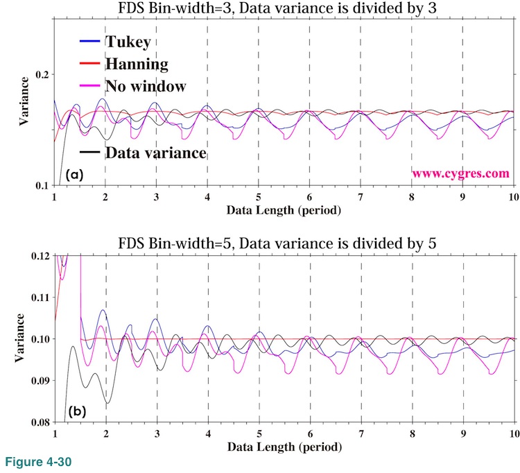
Figure 4-30(a) shows how signal bin variance (PSD of signal bin multiplied by the frequency bandwidth of a bin) and data variance vary as we add more data when 3-bin FDS is applied. The data we used here contains single frequency sinusoid but nothing else and exactly the same as the one shown in Figure 2-4(a). We divided data variance by 3 so that we can compare data variance directly with other values. If we compare this graph with Figure 4-24(b), we can see that FDS considerably reduced deviation of signal bin variance from data variance. Figure 4-30(b) shows the case when we made width of FDS larger. These graphs show that FDS works well to smooth PSD. Please note that the reduction of PSD is reasonable because frequency bandwidth of bins should be modified if we apply FDS as we will describe in (4-3-3). In any case, even though PSD of signal bin becomes smaller, equation (1) still holds because reduction of PSD of signal bin is compensated by increase of PSD of other nearby bins.

(4-3-2) FDS does NOT work well for amplitude spectrum
We showed what would happen if we apply FDS to amplitude spectrum in (2-1-3-3) (Figure 2-10, Figure 2-17). Let us explain why FDS does not work well for amplitude spectrum when window is not applied first. Figure 4-31(a) shows how amplitude of the signal bin varies when we applied 3-bin FDS as we add more data. Here, data contains only a single frequency sinusoid but nothing else as before. This graph is the same as Figure 2-10(a). To explain why the signal bin amplitude becomes larger than the correct value (black horizontal line; 1/3 of actual signal amplitude) when frequency of the signal bin does not match actual signal frequency, let us chose the case when data length is B in Figure 2-4. The data length B is indicated by a short vertical solid black line in Figure 4-31(a). The expanded view of amplitude spectrum near the signal in this case is shown in Figure 4-31(b). The horizontal positions of plus (+) marks in this graph show the frequencies of bins and the horizontal position of vertical solid black line indicates signal frequency. The result of 3-bin FDS of the amplitude of Bin 2 is the simple 3-point average of amplitudes of Bin 1, Bin 2 and Bin 3. Amplitudes of these bins are about 0.18, 0.90 and 0.31, respectively. Then, the average of these is (0.18+0.90+0.31)/3=0.46. Figure 4-31(c) shows reproduced time series of these bins (components of equation (3)). This graph indicates that variations of these components are not aligned but that is not really a surprise because frequencies and phases of these bins are all different. The problem of getting correct amplitude using FDS when frequency does not match, thus amplitudes of Bin 1 and Bin 3 are not 0.0, is that FDS ignores the differences of frequencies and phases of bins. Now we add these three time series together and let us call the result a synthesized time series. Figure 4-31(d) shows this synthesized time series (blue) and the data (purple). Synthesized time series contributes about 93% of data in term of variance. This graph shows that the amplitude of this synthesized time series is about the same as the amplitude of data, 1.0, but it is far smaller than the simple sum of amplitudes of three bins, 0.18+0.90+0.31=1.38.

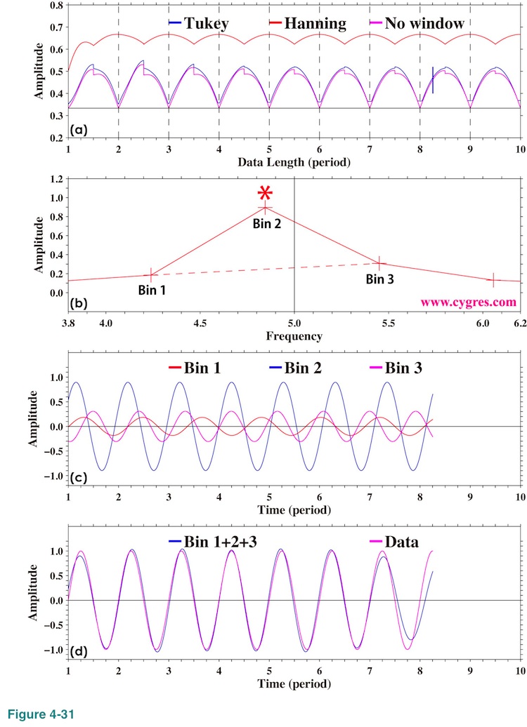
When frequency of the signal bin matches actual signal frequency (data length A in Figure 2-4), the amplitudes of Bin 1 and Bin 3 become zero. Figure 4-32(a) shows time series of data in this case. Amplitude of Bin 2 is equal to the actual signal amplitude (1.0) as shown in Figure 4-32(b). Thus, simple 3-bin average is 1/3 in this case.

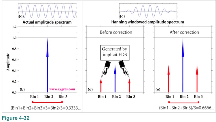
Now, let us show why Hanning windowed amplitude spectrum becomes vastly larger than non-windowed amplitude spectrum when we applied FDS. For the sake of simplicity, let us chose data length to be data length A, so that frequency of signal bin matches actual signal frequency and there is no spectral leakage. Figure 4-32(c) shows time series of data when we applied Hanning window. If we applied Hanning window, width of signal becomes wider as we described in (4-2-6) and now amplitudes of bin 1 and bin 3 are no longer zero as shown in Figure 4-32(d). The correction we described in (4-2-8) brings amplitude of bin 2 to the value almost equal to actual signal amplitude, 1.0, but it also amplifies amplitudes of Bin 1 and Bin 3 as shown in Figure 4-32(e). As a result, simple 3-bin average becomes about 2/3, which is about two times larger than the value when window is not applied. This is why Hanning windowed amplitude spectrum becomes vastly larger than non-windowed amplitude spectrum when we applied FDS.

Thus, in general, FDS does not produce meaningful result for amplitude spectrum and this is why we do not write amplitude in our product file when we applied FDS.

(4-3-3) Frequency resolution when we applied FDS
If we apply FDS, it is reasonable to think that the frequency resolution of resultant PSD should also be modified. Our n-bin FDS is a simple n-bin average and thus it is more natural to think that the frequency bandwidth of the resultant PSD is n times larger than the frequency bandwidth of original PSD. For example, in the case of 5-bin FDS shown in equation (25), it makes sense to pick up only Po(0) (uses Pi(0)~Pi(2)), Po(5) (uses Pi(3)~Pi(7)), Po(10) (uses Pi(8)~Pi(12)),..,Po(5xk; k=any positive integer),... but discard all others, and to make a frequency bandwidth 5 times larger. Alternative choice is picking up Po(2) (uses Pi(0)~Pi(4)), Po(7) (uses Pi(5)~Pi(9)), Po(12) (uses Pi(10)~pi(14)),..., Po(5xk-3; k=any positive integer),... but discarding all others. By doing so, PSD becomes smaller when we applied FDS but the frequency bandwidth becomes larger. This makes that the signal bin variance, PSD of signal bin multiplied by the frequency bandwidth, will not change by FDS, for example.

The primarily reason why we do not discard any of Po is that it would be convenient when we want to import our product file into applications for drawing graphs and/or doing further analyses. Another reason is that we can use intermediate Po such as Po(1) and Po(2) as interpolated Po between Po(0) and Po(5).

(4-3-4) Alternative method of FDS
Welch's method we described in (2-1-3-6) is also widely used to smooth PSD. At this moment, we do not have a plan to include that method in this package deal service. However, if you wish to use Welch's method instead of FDS, please contact us.

(4-4) Percentage of confidence interval; any positive value larger than 0.0 and smaller than 100.0; Default is 95.0
Our customer can choose any percentage value between 0.0 and 100.0 excluding 0.0 and 100.0. Commonly used percentage values are 80%, 90%, 95%, 99% and 99.5%, and we would recommend to choose one among these values unless you have a specific reason to choose otherwise.

Appendix 1; About numerical error generated by computers.
Numerical computations almost always produce some small computational errors in the process. This is because computers assign a memory of fixed size to each numbers they produce in the computational process and some numbers, such as the result of 1/3, are truncated so that they can be stored in a fixed sized memory. To demonstrate how this error is produced, let us assume we have a hypothetical computer, which always assigns a memory that can store 4 digits, this we call significant digit, to any number. Now let's compute (1/3-0.33)x100 from left to right with this computer. The result of 1/3 is 0.3333 or 3.333E-1. Now, subtract 0.33 from it. The value 0.33 is 0.3300 for our computer because significant digit is 4. The result of subtraction is 0.0033 or 3.3E-2. This will not be 3.333E-2 and now we have only two meaningful digits instead of four. Multiplying this by 100, we will get 0.3300 or 3.300E-1. Now let's do this computation manually. (1/3-0.33)x100=(1/3-33/100)x100=(100-99)/300x100=1/300x100=1/3. If we skip all the processes in the middle but just compute the last of this, 1/3, with our hypothetical computer, result will be 0.3333 as before. Comparing this result with the previous result, 0.3300<->0.3333, we see that our computer generated computational error, 0.0033 during previous computation. In our actual computations we have 'about' 16 significant digits. The reason why we have to use a word 'about' is that computers do their business using binary numbers while we human use decimal numbers.

What we would like to say here is that it is reasonable to think that the values of purple and red lines outside of the signal peak in Figure 2-5(a) are zero although actual numbers are not zero.

Appendix 2; Spectral leakage of power spectrum density function and window functions.
We described that spectral leakage occurs if we cannot achieve frequency match because signal bin alone cannot represent actual signal due to the frequency difference, and other bins are needed to hold equation (3) in (2-1-3-3). This is correct but, then, we might ask if using equation (3) is appropriate or not in that case. Our description in (2-1-3-3) merely indicates spectral leakage is not caused by computational error.

In (4-2-1) we described that the 'cliff' at boundaries generated by the assumption of repetition of data (Figure 4-14(b)) is a cause of spectral leakage. The assumption we described there is consistent with the method we and many other people use to compute PSD and the explanation of the cause of spectral leakage is reasonable. However, it only gives us an idea how spectral leakage is generated but we cannot evaluate how large generated spectral leakage would be. Also we will have a problem explaining why we still have spectral leakage even after we applied a window function to remove 'cliffs'.

In this appendix we first introduce alternative way of looking at our limited length data. After that we show how spectral leakage is generated and how large they would be. Finally we describe how to reduce spectral leakage. The root cause of spectral leakage is the fact that the length of our data is limited.

(1) Alternative way of looking at our limited length data
Now let us introduce a new assumption. First, let us assume our data is a portion of infinitely long "Original data" x(n) shown in Figure A2-1(a).

We do not assume repetition of data described in (4-2-1).  Then we apply a window function w(n) shown in Figure A2-1(b) to this infinitely long data.  This window function is called a Boxcar window function due to its shape.  The result is "Our data 2" shown in Figure A2-1(c).  At this point all we need to know about "Original data" is the values between t=0 and T and we know them because our data covers that duration.

We can construct "Our data 2" in Figure A2-1(c) in a different way.  We start from our limited length data x'(n) shown in Figure A2-2(a). This is the exact copy of the one we showed in Figure 4-14(a).

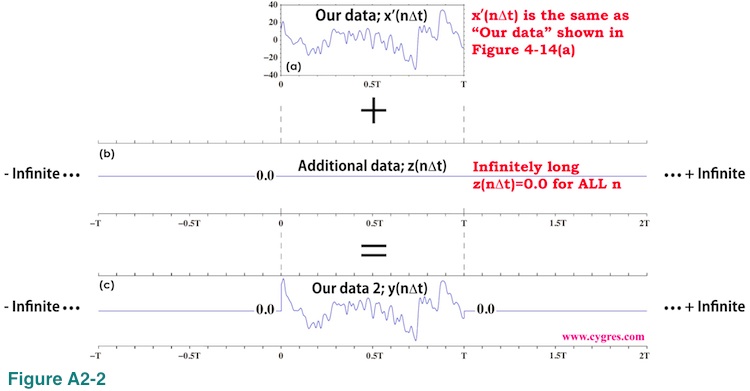
Then, we add infinitely long "Additional data" z(n) shown in Figure A2-2(b) to "Our data" x'(n). All the values of z(n) are zero. Since Fourier transform of z(n) is also zero for any frequency, adding z(n) to "Our data" x'(n) would not modify spectral characteristic of x'(n) at all. By adding z(n) to x'(n), we will get "Our data 2" y(n) shown in Figure A2-2(c). This "Our data 2" is exactly the same as the one shown in Figure A2-1(c). As we described before, we can add any number of data, value of which is exactly zero, to data we want to analyze in order to adjust data length so that we can achieve frequency match. We called it "zero padding". What we did here is the extreme form of zero padding.

The reason why we introduced these two methods to generate identical infinitely long data, "Our data 2", is that we will describe spectral leakage as a deviation of spectral of "Our data 2" shown in Figure A2-1(c) (and Figure A2-2(c)) from spectral of infinitely long data shown in Figure A2-1(a). The latter of which is consdered to be a "true" spectral. This approach makes sense because, although "Our data", limited length data shown in Figure A2-2(a), is what we usually have, spectral characteristic of it is the same as the spectral characteristic of "Our data 2". In other word, we consider limited length "Our data" as a result of the application of a Boxcar window function to an infinitely long data in this appendix. This leads us that if we study how changing the width of a Boxcar window function would affect spectral of resultant windowed data (Figure A2-1), then we would know how changing the data length of "Our data" would affect spectral (Figure A2-2). Thus, we will show how changing the width of a Boxcar window function would affect spectral of resultant windowed data in this appendix.

We cannot evaluate power spectrum density of "Our data 2" at discrete frequencies anymore because data length of "Our data 2" is infinite and frequency bandwidth of bins becomes zero (=1/infinite). Instead of using PSD we introduce similar quantity called PS for infinitely long data as follows. First we extend the range of summation in equation (18) as

For Boxcar windowed data, "Our data 2 (y)" in Figure A2-1(c), equation (A2-1) becomes

The transition from the one marked by blue underline to the one marked by red underline is possible because wm equals zero if m is less than 0 or greater than N-1 and equals 1 otherwise. Please note that rightmost part (red underline) of equation (A2-2) is the same as equation (18) except for the frequency. Since we can compute Yr and Yi at any frequency, we can compute them at frequencies where we computed PSD in section (2). In that case, the rightmost part of equation (A2-2) will be exactly the same as equation (18).

Using Yr and Yi we define a quantity PS for infinitely long data as

This quantity PS is very much similar to PSD (equation (19)). One of the apparent differences is that there is no multiplication factor 2.0 in equation (A2-3). This is because we want to define PS both at positive and at negative frequencies. Another apparent difference is that equation (A2-3) is not divided by T but this is simply because T is infinite for infinitely long data. Aside from these apparent differences, the most important difference between PS and PSD is that PS is continuous in frequency and this becomes very convenient to understand why spectral leakage occurs.

Actual values of PS of "Our data 2 (y)" in Figure A2-1(c) divided by T (equals width of a Boxcar window function) and multiplied by 2 at frequencies where we ordinarily compute PSD are exactly the same as PSD of "Our data (x')" in Figure A2-2(a). This is because equation (A2-2) will be exactly the same as equation (18) in that case as we described before.

(2) How spectral leakage is generated and how large it would be
In the case when we need to deal with real world data, we usually cannot compute equation (A2-1) because it is usually not possible to have infinitely long data. However, in the case when we use hypothetical data we might be able to mathematically evaluate equation (A2-1). In the following we use hypothetical data we used in Case 1, (2-1-3-3), namely,

In this case Xr(f) and Xi(f) are

Equation (A2-5) shows that the Fourier transform of x(t) is non-zero only at two specific frequencies. Using the result of this and the convolution theorem we described in (4-2-6), we can evaluate middle part (blue underline) of equation (A2-2) as follows.

Here W(f) is the Fourier transform (discrete) of a Boxcar window function,

k in the second line is an integer, greater than 0 and less than N/2+1.

The last part of equation (A2-6) (red underline) show that Fourier transform of Boxcar windowed x(t) is quite different from Fourier transform of x(t) shown by equation (A2-5). This difference is caused by spectral leakage. Decomposing W in equation (A2-6) into a real part (Wr) and an imaginary part (Wi) and substituting them into equation (A2-3), PS of the Boxcar windowed data is,

To show how the spectral leakage occurs by showing the convolution process graphically we have chosen two different cases. Figure A2-3(a) shows time series plot of data (Equation (A2-4)) we have used. Each data is shown as a small dot in this graph and we connected dots by straight blue lines.

The first case (Window-width A) is when window-width is 40 (data points). This is the case when frequency match is achieved and this case is equivalent to the data length A shown in Figure 2-4. From this graph we might get an impression that the second cycle is not completed in this case but the zero value point next to the end point is actually the start point of the next cycle and does not belong to the second cycle. Another case (Window-width B) is when window-width is 50 and this case is similar to the case of data length C in Figure 2-4. We intentionally made these window-widths rather narrow so that following graphs are easy to see. In the following A in equation (A2-4) (amplitude of x(t)) is 1.0 and the sampling interval is 0.05, which results that fundamental frequency range is -10 to 10.

Before showing how the convolution process works we show PS for infinitely long Boxcar windowed data similar to "Our data 2" in Figure A2-1(c) and PSD for limited length data similar to "Our data" in Figure A2-2(a) first. The red line in Figure A2-3(b) shows PS of Boxcar windowed infinitely long data x(t) for the case A. Since data length is infinite, we can evaluate continuous PS. We omitted PS in the negative frequency range because PS is symmetrical with respect to the zero frequency. The vertical blue arrow in this graph is PSD of limited length data multiplied by T and divided by 2 and we call it modified PSD. It is no accident that the tip of this arrow touches PS (red line). The values of modified PSD (blue arrow) and PS (red line) at the same frequency must be the same as we described before. Since this is the case when frequency match is achieved, PSDs of bins are zero except for a signal bin as we showed in Figure 2-5(a) (Purple line; "No window" case). Thus, there is only one blue arrow in this graph and the signal frequency shown by a short green solid line matches frequency of that arrow. The vertical dashed blue lines indicate frequencies of other bins. PS at those frequencies is zero from the second line of equation (A2-7) because both f1 and f2 of equation (A2-6) become integer multiples of 1/T at those frequencies.

Figure A2-3(c) shows PS and modified PSD for the case B. Since PSDs of all the bins are non-zero due to the spectral leakage, we omitted vertical dashed blue lines in this graph. The solid blue line (labeled as "Envelope") connecting tips of the arrows shows that the result shown in this graph is similar to the PSD shown in Figure 2-6(c) (Purple line). Again, values of modified PSD and PS at the same frequency are the same (tips of arrows always touch red line). Figures A2-3(b) and (c) suggest that spectral leakage always occurs but we do not see it on graphs of PSD when we achieved frequency match because the effect of spectral leakage is zero at frequencies where we ordinarily compute PSD for that case. It is slightly difficult to see but the PS of the main lobe is not symmetrical with respect to the center of the main lobe. Due to this asymmetry the bin of the maximum amplitude may not be a signal bin when we cannot achieve frequency match as we described in (2-1-3-3).

Now let us show how the spectral leakage occurs by showing the convolution process graphically. We picked up bins marked by purple solid triangles labeled fT in figures A2-3(b) and (c) for this purpose. The upper panel of Figure A2-4 shows the Fourier transform of an infinitely long data x(t) and the lower panel of Figure A2-4 shows the Fourier transform of a Boxcar window function.

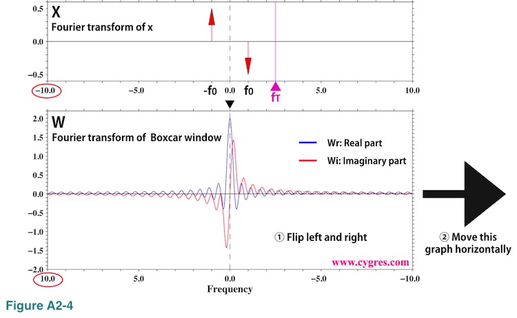
These are graphical representations of equations (A2-5) and (A2-7), and the fundamental frequency ranges (horizontal width of the graph) of these two are the same because sampling interval of infinitely long data x(t) and Boxcar window function w(t) must be the same. There is no real part component in the upper graph of Figure A2-4. To calculate PS at frequency fT (purple solid triangle) using convolution, the first thing we do is flipping lower graph left and right. This is already done in this graph so that frequency (horizontal axis) of the lower graph decreases from left to right unlike upper graph (red circles). The next thing we do is moving this lower graph horizontally so that the horizontal position of the center of lower graph marked by a black solid triangle matches the horizontal position of fT in the upper graph. The result of this manipulation is shown in Figure A2-5. We omitted unnecessary parts in these graphs.

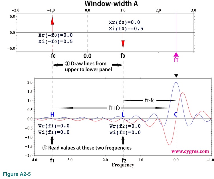
Then, we draw lines vertically from the upper graph to the lower graph at frequencies f0 and -f0 (vertical dashed lines H and L). Since the frequency difference between H and C (rightmost vertical dashed line) is fT-(-f0)=fT+f0=f1 and the frequency difference between L and C is fT-f0=f2, frequencies of these two dashed lines in the lower graph are f1 and f2 (Please see equation (A2-6)). If f1 goes beyond of the edge shown in Figure A2-4, we use periodicity of the Fourier transform as we will show later,

As a fourth step, we read values of blue (real part) and red (imaginary part) lines at places where dashed lines H and L intersect those lines. Then, we calculate X multiplied by W as
XW(f1)={Xr(-f0)Wr(f1)-Xi(-f0)Wi(f1)}+i{Xi(-f0)Wr(f1)+Xr(-f0)Wi(f1)}={-Wi(f1)/2}+i{Wr(f1)/2}
XW(f2)={Xr(f0)Wr(f2)-Xi(f0)Wi(f2)}+i{Xi(f0)Wr(f2)+Xr(f0)Wi(f2)}={Wi(f2)/2}+i{-Wr(f2)/2}
After this we calculate XW(f1) + XW(f2). This is how the convolution process is used to obtain the last part (red underline) of equation (A2-6). Figure A2-5 shows that this computation is similar to the computation of weighted moving average (as we described before, in the strict sense it is not an average because the summation of weights is not equal to 1.0) of X with the weight W as we described in (4-2-6). As a final step, we decompose sum of XW(f1) and XW(f2) into a real part and an imaginary part and then substitute the result into equation (A2-3). This will give PS of Boxcar windowed data at frequency fT,

In case of window-width A shown in Figure A2-5, Wr(f1), Wi(f1), Wr(f2) and Wi(f2) are all zero as we described before. Thus, PS at fT is zero from equation (A2-8). Likewise, PS at frequencies where we ordinarily compute PSD except for signal bin frequency becomes zero and we do not see spectral leakage at those frequencies. However, if we compute PS at any other frequency, we will pick up signal no matter how far away fT is from f0 (signal frequency).

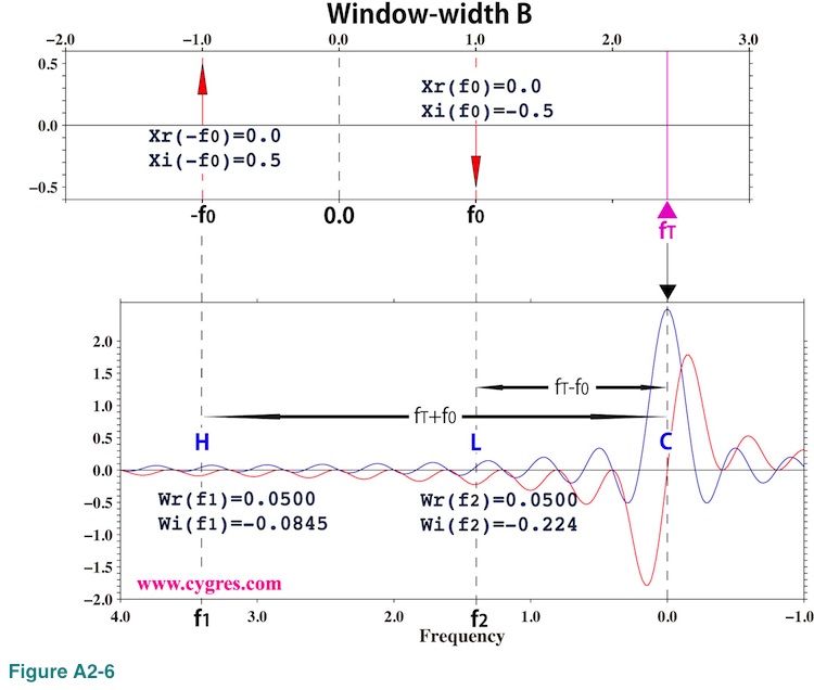
Figure A2-6 shows the case when window-width is B. In this case, none of Wr(f1), Wi(f1), Wr(f2) and Wi(f2) is zero, and as a result, PSD becomes non-zero even if fT is far away from f0.

Equation (A2-8) shows magnitude of spectral leakage at any frequency is determined by the Fourier transform of a window function. Lower part of Figure A2-4 shows that the value of the Fourier transform of a Boxcar window function oscillates and the amplitude of this oscillation decreases as frequency deviates away from zero in either direction. This results that the magnitude of spectral leakage tends to become smaller as the difference between fT and f0 becomes larger. However, spectral leakage will never be zero in this case.

Figure A2-7 shows convolution process for general cases when the Fourier transform of infinitely long data (X in Figure A2-7(a)) is more complicated than the one we have shown so far.

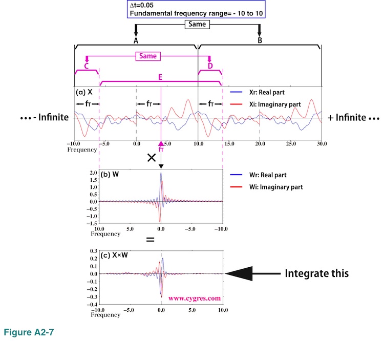
In this graph we show segment A covering fundamental frequency range and segment B, frequency width (horizontal width in this graph) of which is the same as frequency width of segment A. The contents of these two segments are identical due to the periodicity of X we described before. Let us assume we want to compute PS at frequency fT (purple triangle) as before. We shift horizontal position of the graph of the Fourier transform of a Boxcar window function (W in Figure A2-7(b)) after flipping it left and right as before. Here, the frequency width of W is the same as the frequency width of segment A.

For the convolution we chose segment E of X. The frequency width of segment E is the same as frequency width of segment A. The segment E lacks the segment C of segment A at left but the segment D of segment B added at right compensates this missing segment. Again, due to the periodicity of Fourier transform, contents of segments C and D are identical. In this way, the extent of convolution covers entire fundamental frequency range of X no matter where fT exists. We multiply segment E of X by W in the same way we did in figures A2-5 and A2-6; multiply two values at the same horizontal position together. The result of this multiplication is shown in Figure A2-7(c). Then we integrate (sum) this result to obtain Yr(fT) and Yi(fT) to compute PS at frequency fT using equation (A2-3). These graphs clearly show that the convolution is similar to the weighted moving average (in the strict sense it is not an average because the integral of weight is not equal to 1.0) of X with the weight W and the width of averaging is equal to the fundamental frequency range. As a result, PS at any frequency fT would pick up all the signals on X except for those at frequencies f that satisfy fT - f = +/- k/T (second line of equation (A2-7)).

(3) How to reduce spectral leakage
If we have infinitely long data, we will not have spectral leakage, but of course, length of our real world data is always limited. Alternatively, if we can achieve a frequency match, we can remove spectral leakage but it is usually impossible to achieve a frequency match when we need to deal with real world data. Then, what we actually can do to reduce spectral leakage is proactively choosing a window function that would reduce spectral leakage instead of accepting a Boxcar window function that would be applied automatically if we do nothing. As we have shown already, the magnitudes of spectral leakage would decrease if the magnitudes of the Fourier transform of a window function at frequencies other than zero become smaller. A window function which is infinitely wide (long) and all the values are 1.0 will prevent spectral leakage completely. However, in order to apply a window function like that, we need to have infinitely long data because length of data must be equal to width of a window function. Thus, that is not a practical solution.

As an example of an alternative window function we use a Hanning window function here. The Fourier transform (discrete) of a Hanning window function is

k in the third line is an integer, greater than 1 and less than N/2+1.

Figures A2-8(a) and (b) show Fourier transform of a Boxcar window function and a Hanning window function, respectively.

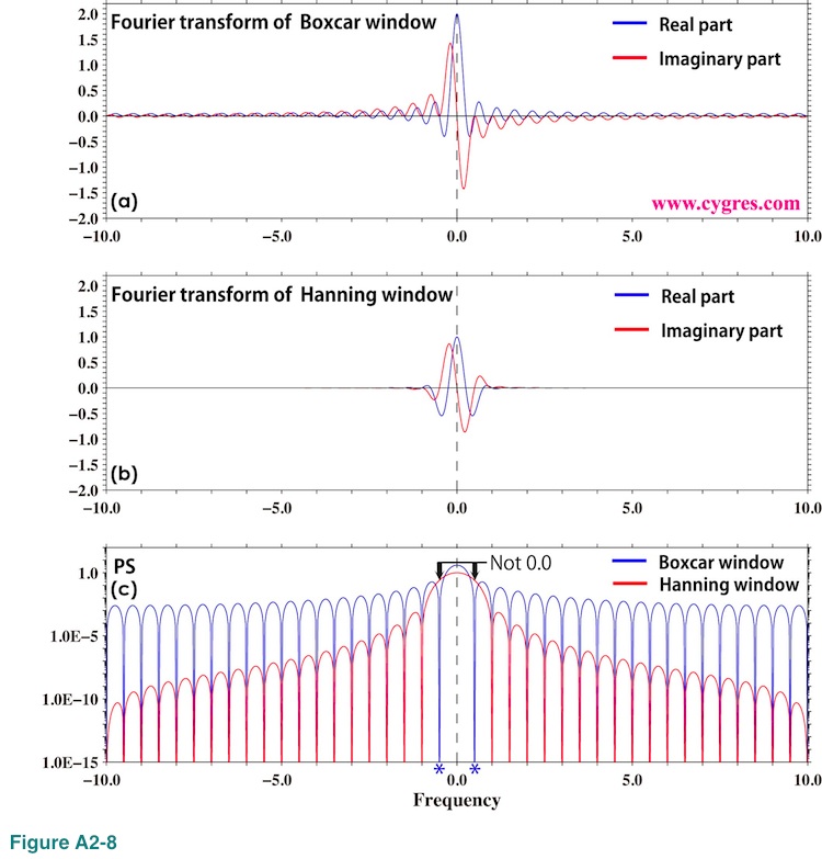
While we can see blue and red lines clearly over entire frequency range in Figure A2-8(a), it is difficult to see those lines beyond of +/- 2.0 in Figure A2-8(b). Figure A2-8(c) shows PS of these two windows. Please note that we used logarithmic scaling for this graph unlike others. From this graph we can see that Hanning window would considerably reduce spectral leakage and reduction rate would progressively increase as the difference between fT and f0 (Figure A2-4) becomes larger. This graph also shows that, although applying Hanning window removes 'cliff' described in (4-2-1), we will still have spectral leakage.

Another thing we can see in this graph is that while the PS of a Boxcar window function at frequencies marked by blue asterisks is zero, PS of a Hanning window function is not zero at those frequencies. Also, PS of a Hanning window function at zero frequency (black dashed vertical line) is smaller than the PS of a Boxcar window function at that frequency. These are the cause of widening of signals when we applied a Hanning window function as we described in (4-2-6).

These results suggest that it would be better if we apply Hanning window before computing PSD. However, a Hanning window function and many other window functions considerably dump significant portion of data. In certain cases, applying these window functions may cause a problem as we described in (4-2-3).

(4) Alternative method to reduce spectral leakage (Not supported in this package deal service)
An alternative method to reduce spectral leakage is to use a method called Maximum Entropy Method (MEM hereinafter). We will use weak signals SR shown in Figure 4-9(a) and a strong sinusoidal signal S1 similar to the one shown in Figure 4-9(c) to demonstrate the effectiveness of spectral leakage removal by MEM. Although there are several different methods categorized as MEM, we will only demonstrate results of MEM developed by Dr. Burg. At this moment we do not have an intention to implement MEM in PD001A/B.

We will start showing that the overall general characteristic of PSD of data, that contains various signals and noises such as SR, computed by MEM is quite similar to the overall general characteristic of PSD computed by PD001A/B. Figures A2-9(a) and (b) show PSDs of SR computed by PD001A/B (blue and red lines) and by MEM (purple lines). We moved blue and red lines upward to make comparison easier. The data, SR, we used here is the same as the one shown in Figure 4-9(a). The number of data is 8514 and this is the case when spectral leakage caused by S1 would be close to the maximum if we add S1 and use PD001A/B to compute PSD (similar to "Window-width B" in Figure A2-3 or "data length C" in Figure 2-4(b)). We did not detrend data for the sake of consistency. There are two peaks labeled S2 and S3 in these graphs. We use these two peaks as targets to detect as before because variations represented by these peaks are tidal components and they exist relatively steadily throughout the entire record of SR.

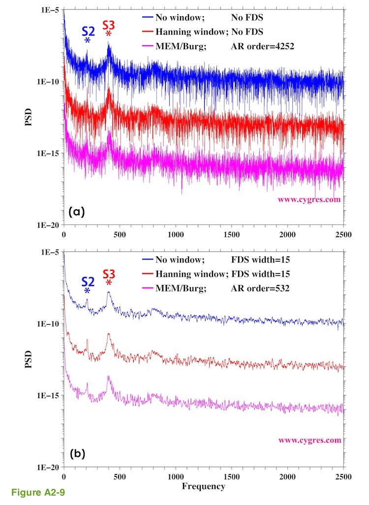
The blue line in Figure A2-9(a) shows the case when we did not apply any window function and it is the same as the black line shown in Figure 4-13(a) except that we used linear horizontal axis this time and we moved the line vertically. The red line in Figure A2-9(a) shows the case when we applied Hanning window and it is the same as the black line shown in Figure 4-13(c). The difference between Figure A2-9(a) and A2-9(b) is that the results shown in Figure A2-9(a) are the cases when we did not apply FDS and the results shown in Figure A2-9(b) are the cases when we applied FDS. FDS has an effect of smoothing PSD as we described in (4-3).

The purple lines in Figure A2-9(a) and A2-9(b) show PSDs computed by MEM. There is a parameter called autoregression order (AR order) when we compute PSD by MEM and it affects practical frequency resolution among others. We adjusted AR orders so that resultants PSDs would have similar practical frequency resolutions to those of others in Figure A2-9. We can compute PSD at arbitrary frequencies if we use MEM but we computed PSD at the frequencies where we would compute PSD if we use PD001A/B (blue and red lines) for the sake of comparison.

The point we would like to make here is that figures A2-9(a) and A2-9(b) show that overall general characteristics of PSDs of SR computed by these different methods are quite similar. After all, we are trying to compute same thing, PSD. However, if we take a close look at these graphs we will see the differences. For example, PSD computed by MEM suggests S3 might include signals of several slightly different frequencies, which is quite possible because S3 corresponds to semi-diurnal tide, and semi-diurnal tide is known to have several components at slightly different frequencies. Likewise, some of these differences of PSDs of SR might become very important for serious spectral analyses but we will ignore these differences in this Appendix.

The blue lines in Figure A2-10 show PSDs when S1 is added to SR and the black lines in Figure A2-10 show PSDs of SR alone. Figure A2-10(a) shows PSDs computed by PD001A/B when we did not apply any window (equivalent to applying Boxcar window) and Figure A2-10(b) shows PSDs computed by PD001A/B when we applied Hanning window. Figure A2-10(c) shows PSDs computed by MEM. We did not detrend data for these computations and we moved black lines downward to make comparison easier. The blue line in Figure A2-10(a) is the same as the blue line in Figure 4-13(a) and the blue line in Figure A2-10(b) is the same as the blue line in Figure 4-13(c) except that we used linear horizontal axis this time. The black lines in Figure A2-10(a), (b) and (c) are the same as the blue, red and the purple lines in Figure A2-9(a) except that we moved some lines vertically.

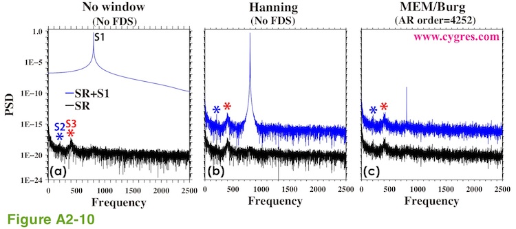
Figure A2-10(a) shows that spectral leakage of S1 practically makes it impossible to detect SR if we did not apply any window. Figure A2-10(b) shows that spectral leakage of S1 is reduced considerably by Hanning window but existence of it is still obvious. MEM, by principle, produces no spectral leakage by windowing and, Figure A2-10(c) clearly shows it.

Now, let us take a look at S1 instead of SR. The PSDs of S1 shown in Figure A2-10(a) and A2-10(b) are reasonably close to the actual PSD of S1. On the other hand, PSD of S1 shown in Figure A2-10(c) is considerably smaller (about 1/500000000) than the actual PSD of S1 although PSDs of S2, S3 and others of SR are comparable to those in Figure A2-10(b). This is mostly because we did not compute PSD at the frequency of S1 (800) although S1 is a constant amplitude and constant frequency pure sinusoid without any phase variations. To make this point clearer we recomputed PSD with a much smaller frequency interval. The blue (SR+S1) and the black (SR alone) "x" marks in Figure A2-11 show the results of these recomputations. Please note that the frequency range of this graph is only between 785 and 815.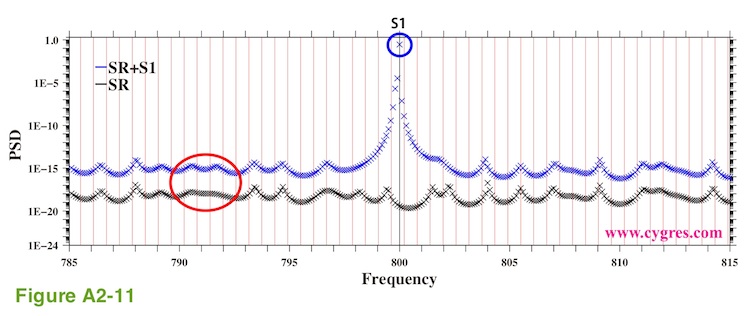

The vertical red lines in this graph indicate frequencies where we computed PSD in Figure A2-9(c) and the vertical black line at the center of this graph indicates frequency of S1. One of the frequencies where we computed PSD this time exactly matches the frequency of S1 and the blue "x" mark at the center of the blue circle labeled S1 shows PSD at the frequency of S1. This value is reasonably close to PSD of S1. Ideally, we should not be able to see S1 except at the exact frequency of S1 but we can see S1 in Figure A2-10(c) because MEM gives non-zero frequency width to S1 (S1 is not a "line" but a steep "mountain") as shown in Figure A2-11. Nevertheless, this graph suggests that we need to choose frequencies where we compute PSD carefully if it is important to know magnitudes of PSD of signals when signals are similar to S1, a constant amplitude and constant frequency pure sinusoid without any phase variations. If the magnitude of S1 is comparable to those of S2 and S3, we might even miss S1. However, if amplitude of S1 varies, theoretical peak of PSD due to S1 will have some frequency width as we described in (Case 3) of (2-1-3-3).

The horizontal scale of "hills" and "valleys" shown by "x" marks in Figure A2-11 is about the same as horizontal distance between adjacent vertical red lines. Thus, the frequency interval of PSD computations we chose for Figure A2-11 is apparently much smaller than the actual frequency resolution of PSD. Frequency resolution of PSD computed by MEM is determined by AR order and there is a limit determined by sampling interval and number of data. Computing PSD with smaller frequency interval as we did may help obtaining peak frequencies accurately but it does not necessarily give us PSD of a finer frequency resolution. Another thing we would like to mention is that, while MEM does not leak spectrum, we still can see the effect of S1 (red ellipse) away from the "mountain" of S1.

Since MEM does not assume that data is composed of pure sinusoids unlike PD001A/B (please, see equation (3)) MEM occasionally gives us unexpected results when data is consist of pure sinusoids as in the case shown in (2-1-3-3). We generally recommend computing PSDs by several different methods and comparing results for serious spectral analyses.

Appendix 3; Why we see a single peak instead of twin-peaks when data length is short.
We described in the Example 1, (Case 3-1) that when the amplitude of single frequency sinusoid varies sinusoidally we would see a single peak if data length is short and we would see two peaks (twin-peaks) when data length is long. This behavior can be mathematically explained by the Convolution theorem, which dictates that Fourier transform of the product of two functions (S0 and S1; first expression of equation (4)) is equal to the convolution of Fourier transform of individual functions. As we described in (4-2-6) we compute PSD and amplitude spectrum using results of Fourier transform of data. For more about Convolution theorem, please see (4-2-6).

When data is short relative to the period of S1, f1 will be included within zero-frequency bin because frequency bandwidth of bins (frequency resolution) is so large. Then, convolution would not modify frequency of S0 and the peak of PSD of our data will be at f0. At this stage, data is practically S0 except that amplitude is very, very slowly varying. Please note that this data length is short relative to the period of S1 but it is fairly long relative to the periods of SL and SH as shown in Figure 2-11.

As we increase data length, frequency resolution of the Fourier transform becomes finer and f1 leaves from zero-frequency bin but moves toward higher frequency bin. Then, convolution of the Fourier transform of S1 and the Fourier transform of S0 starts generating twin-peaks center of which is at f0.

The alternative way of understanding why we need more than certain length of data to have twin-peaks is considering this as a problem to separate two neighboring singnals, frequency difference between them is 2 x f1.

Appendix 4; How the frequency of S1 affects the detectability of SR
Let us assume that S1 in Figure 4-9 is a sinusoid of amplitude G and the frequency of it is the same as the frequency of k-th bin (frequency match is achieved). Let us also assume that SR is a sinusoid of amplitude A and frequency of it is the same as the frequency of m-th bin. The latter assumption makes PSD of SR zero except for m-th bin. In this case the ratio of the PSD of SR to the PSD due to added 'inclination' at the m-th bin is, from equation (17) and equation (14),

Now let us assume that the case when PSD due to added 'inclination' significantly affects the detectability of SR is the case when above ratio is less than 1.0. Using equation (A4-1) this condition can be expressed in term of amplitude ratio of SR (A) to S1 (G) as

Above equation shows that if frequencies of both S1 and SR are low (thus, both k and m are small), it would be difficult to detect SR even if amplitude of SR is relatively large.

In case of the example we showed in Figure 4-10, k is 8. Substituting this value into (A4-2), the ratio A/G when the PSD of SR is equal to the PSD due to added 'inclination' is 0.076/m. This means that, if amplitude of S1 (G) is 1.0, amplitude of SR (A) must be 0.076 for m=1 and 0.00076 for m=100 so that PSD of SR at m-th bin is equal to the PSD due to added 'inclination' at m-th bin.

On the other hand, k is 1600 for the example we showed in Figure 4-12. In this case, the ratio A/G when the PSD of SR is equal to the PSD due to added 'inclination' is 0.00038/m. If m is greater than about 120 (corresponding frequency is about 74) or so, PSD of SR becomes comparable to the PSD due to added 'inclination'. As a matter of fact we can see SR in the right half of Figure 4-12(d).

END of User Guide of PD001A (Copyright: Cygnus Research International, Apr. 21, 2014)

To read previous page, please click button below.