Power Spectral Density computation (Spectral Analysis)
MicroJob Package Deal Service PD001A/B(Copyright Cygnus Research International (Apr 20, 2015))

Page 5 of PD001A/B User Guide

Table of Content
(1) Summary of PD001A/B
(1-1) What this Package Deal service, PD001A does
(1-2) What PD001B does
(1-3) Summary of selectable computational parameters
(1-3-1) Detrending data (Applicable to all cases)
(1-3-2) Confidence interval percentage (Applicable to all cases)
(1-3-3) Taper ratio of a Tukey window (Applicable to cases B1, B2 and B3 only)
(1-3-4) FDS bin-width (Applicable to all cases except for cases A1, B1 and C1)
(1-4) Computational procedure
(1-5) Your Data (Input data)
(1-6) Products
(1-6-1) Data file (Product file)
(1-6-2) Graphs (Figures) in PDF (PD001A only)
(1-7) Price and ordering procedure
(1-8) Confidentiality
(2) Detail of the product
(2-1) Product files
(2-1-1) Format of Product file
(2-1-2) Explanation of contents of product files
(2-1-2-1) Frequency
(2-1-2-2) Period
(2-1-2-3) PSD
(2-1-2-4) Confidence interval of PSD
(2-1-2-5) Percent of variance
(2-1-2-6) Amplitude (Amplitude spectrum)
(2-1-2-7) Phase
(2-1-3) How to use/interpret data in our product file
(2-1-3-1) Drawing graphs
(2-1-3-2) PSD and Confidence interval of PSD
(2-1-3-3) Estimating amplitude of variations at specific frequencies using amplitude spectrum
(Case 1) When the signal is a sinusoid and the amplitude of it is constant or almost constant in time
(Case 2) When the signal itself is not a sinusoid but the composition of sinusoids of various frequencies
(Case 3) When the signal is sinusoid but the amplitude of the signal varies in time
(Case 3-1) Variation of amplitude itself is sinusoidal
(Example 1) Amplitude of sinusoidal oscillation of frequency f0 varies sinusoidally.  Frequency of amplitude variation is f1 and f1 is smaller than f0. Both f0 and f1 are constants.
(Example 2) Amplitude of sinusoidal oscillation of frequency f0 is summation of a constant and a sinusoidal variation of frequency f1.
(Case3-2) Amplitude of sinusoidal oscillation of frequency f0 varies but that variation does not resemble to a sinusoid.
(Case4) When the signal is periodic but the signal does not look like a sinusoid
(2-1-3-4) Obtain some idea how strong the variations within a specific frequency range are.
(2-1-3-5) Construct digitally filtered time series data
(2-1-3-6) Alternative method of amplitude estimation
(2-2) Graph
(3) How to prepare data for this package
(4) Guide for setting proper selectable parameters
(4-1) Detrending and removing average; Yes or No? Default setting is Yes.
(4-1-1) What is detrending? Why do we have to do that?
(4-1-2) Example of detrending
(4-1-3) When detrending becomes harmful
(4-2) Taper ratio of Tukey window; 0~100(%) Default setting is 10%
(4-2-1) Why we need to apply a window function
(4-2-2) What does window function do
(4-2-3) Why Hanning window is not necessarily a good solution
(4-2-4) Why we provide non-windowed and Tukey windowed result for PD001A
(4-2-5) The method to reduce dumping near the both ends of data while still using Hanning window
(4-2-6) Implicit FDS
(4-2-7) Implicit FD'Smoothing' Really?
(4-2-8) Reduction of PSD and amplitude due to the window
(4-2-9) Does correction of reduction of PSD work well?
(4-2-10) Tukey window; how taper ratio affects its characteristics
(4-3) Bin-width of FDS; 1,3,5,7,... (Odd integer); Default setting is None, 3 and 7
(4-3-1) FDS works well for PSD
(4-3-2) FDS does NOT work well for amplitude spectrum
(4-3-3) Frequency resolution when we applied FDS
(4-3-4) Alternative method of FDS
(4-4) Percentage of confidence interval; any positive value larger than 0.0 and smaller than 100.0; Default is 95.0

Appendix 1; About numerical error generated by computers.
Appendix 2; Spectral leakage of power spectrum density function and window functions.
Appendix 3; Why we see a single peak instead of twin-peaks when data length is short.
Appendix 4; How the frequency of S1 affects the detectability of SR

(4) Guide for setting proper selectable parameters
This section is to provide enough information to choose the best parameters for your PSD computations. To achieve this goal we explain some technical details using mathematical equations. If you are considering ordering this package deal service we will be happy to answer your questions before ordering.

(4-1) Detrending and removing average; Yes or No? Default setting is Yes.
In general detrending data before computing PSD is recommended. We will show some (we believe rare) cases when detrending becomes harmful.

(4-1-1) What is detrending? Why do we have to do that?
What we call detrending is that we remove a linear trend, a straight-line least square approximation of data, from data. It is not rare to see very low frequency fluctuations including linear increase or decrease in industrial or engineering data caused by environmental changes such as temperature increase around sensors. Engineers often call that a "drift". The primary purpose of detrending is to remove extremely low frequency, frequency below the first non-zero frequency of PSD, component from data before computing PSD. If we do not detrend data, PSD at low frequency range may become too large. If we actually have a linear trend in our data, effect of it could be spread to entire frequency range as we show later. Another important aspect of detrending is that the average of detrended data becomes zero. Removing average of data, often called DC component or bias by Electric engineers, makes the zero frequency (second row of our product file) PSD zero.

(4-1-2) Example of detrending
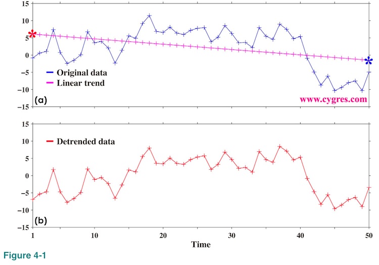
The blue line in Figure 4-1(a) shows data for this example. The plus (+) marks show actual data points. We first compute a linear trend using a least square method. This is to find "Slope" and "Intercept" that minimize "Er" in the equation below.

where N is the number of data, tm is the time of m_th data point (horizontal positions of blue + marks in the graph) and V(tm) is the value of m_th data (vertical positions of blue + marks). The "slope" in this case is

and the 'intercept" is the vertical position of the purple line at t=0, which is one point left (outside) of the left edge of this graph. After computing "slope" and "intercept", we compute linear approximation of data, namely (Slope x tm + Intercept), at each data point. The purple line in this graph is this linear trend. Finally, we subtract this linear trend from data and the result is shown in Figure 4-1(b).

(4-1-3) When detrending becomes harmful
Removing a linear trend almost always works fine but it may become problematic in some rare cases when we try to detect very weak signals in the presence of very strong signals. Here, how weak 'very weak signals' should be relative to 'very strong signals' depends on frequency of signals. The graphs we show below might raise your concern about detrending but we believe this particular problem will be negligible for great majority of cases we will encounter. This problem may become significant if (1) our data has a large number of significant digits, (2) our data contains very weak signals mixed with very strong signals, (3) we need to analyze these very weak signals, (4) effect of spectral leakage of those strong signals is small and (5) noise in our data is much weaker than the weak signals we want to analyze. If condition (1) is not satisfied, we basically cannot have 'very' weak signals. If we are not interested in weak signals to start with (condition (3)) we do not need to care about this problem. If we have a noise, amplitude of which is larger than the weak signals (condition (5)) we will have trouble to detect our weak signals even if there were no strong signals (Figure 2-33). We will show what condition (4) means with some examples later but, first, we will show the cause of the problem.

The blue curve in Figure 4-2(a) shows first one period plus one more point of test data we used in Figure 2-4(a) and this corresponds to V(tm) in equation (13). This is just a minor detail but the reason we added one extra point which is actually the first point of the second period is that the end point of the first period is not the point where blue curve crosses zero but one point before that occurs. We want to have zero-to-zero data here and since our data is discrete (not continuous), we need to have one extra point. Now, our first guess of the linear line approximation, a linear trend, of blue curve is black line; zero slope and zero intercept.

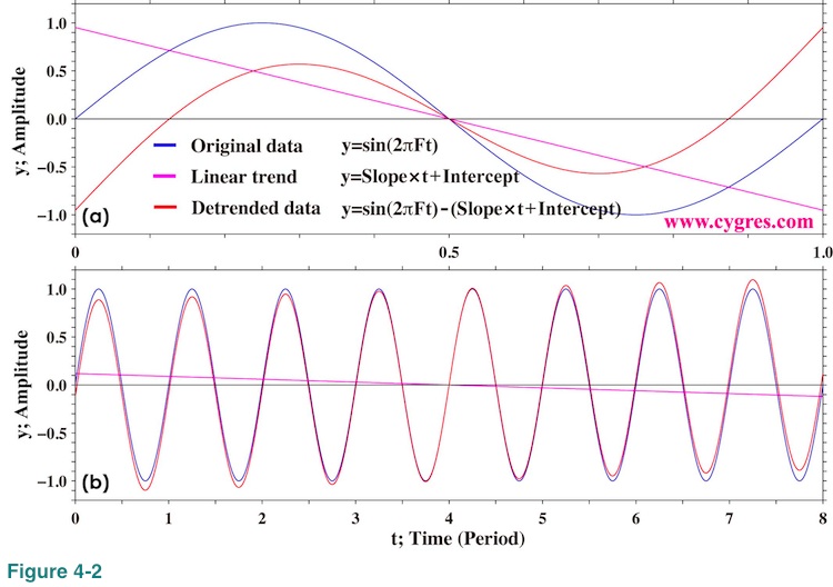
Unfortunately our rather innocent guess turned out to be wrong and an actual linear trend of blue curve using equation (13) is the purple line in this graph. The red curve in this graph shows detrended data. The problem we will describe in this section is that, by detrending a pure sinusoid, we actually add linear 'inclination' component to a pure sinusoid. Please note that PSD computation is based on the premise that our data can be described by summation of pure sinusoids of discrete frequencies and a constant (zero frequency component) as shown by Equation (3). 

Making data length longer does not solve this problem.  Even if we have 8 period lengths of data, corresponding to data length A in Figure 2-4(b), we still have non-zero 'inclination' as shown in Figure 4-2(b). This can be mathematically explained relatively easily by letting sampling interval be very small and then approximating summation in equation (13) by integral. By doing so, slope for the sinusoidal curve of amplitude G, frequency F and phase P, that starts from time=0 and ends at time=T, becomes

If P=0 as in the case shown in Figure 4-2, this equation becomes

We skip all the algebraic detail of getting this equation because it is a tedious book-keeping job and we do not think showing the process of getting this equation will serve the purpose of this document.

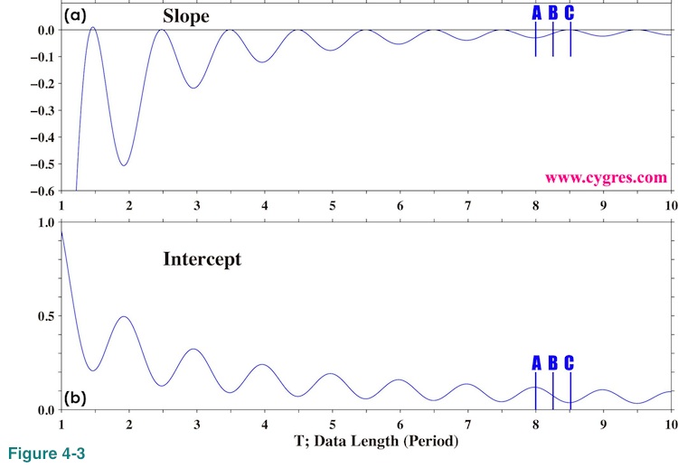
Figure 4-3(a) shows how the slope varies as we add more data when amplitude G is 1.0 and frequency F is 1.0. The unit of horizontal axis of this graph is the period of sinusoid (=1/F). The data lengths A, B and C indicated by vertical short blue lines are the same as those in Figure 2-4(b). If we set start point of our data half a period ahead, result will become a mirror image of this graph with respect to the horizontal black line drawn at 0.

This indicates that slope is almost always negative and it only becomes approximately zero when data length is extremely long or approximately n plus half a period where n is any integer greater than 1. These are clearly seen in Figure 4-3(a). This equation also shows that the magnitude of slope increases as the amplitude of sinusoid increases and decreases as frequency of sinusoid and/or data length increases. With a fixed data length T, slope decreases as frequency of sinusoid increases.

It is ironical enough that we will add 'inclination' to a pure sinusoid by detrending it but the most ironical part of this result is that both slope and intercept of 'inclination' become large when we achieve frequency match (data length A). The accuracy of PSD computation is the best when we achieve frequency match as shown before.

Adding 'inclination' to a pure sinusoid would cause two effects on PSD. Let us call 'a pure sinusoid', signal. The first one is addition of PSD of 'inclination' to the PSD of the signal. If data length is A (end of 8th period; T=8/F), then only a single bin, frequency of which is equal to frequency of the signal (we call it frequency match before), has non-zero PSD if we do not detrend (Figure 2-5(a)) and this is true PSD of this signal. PSD due to the added 'inclination' at k_th bin for data length A is from equation (14),

Here, the amplitude of the signal is equal to 1.0 (G=1.0). We give bin number one to the lowest non-zero frequency bin (third raw of our product file). PSD of zero frequency bin (k=0; second raw of our product file) is zero if we detrend data. This equation shows that PSD due to added 'inclination' increases if frequency of the signal decreases. PSD of the bin where signal exist in this particular case (data length=A) will be simply adding result of equation (17) to true PSD of the signal which is equal to the variance of signal divided by frequency bandwidth of bin.

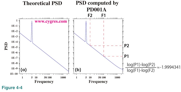
Equation (17) also shows that if we draw this PSD on a logarithmically scaled graph we will see a straight-sloped line since frequency, f, of k_th bin is k/T. Taking the log of both sides of equation (17),

Figure 4-4(a) shows PSD obtained from above equations and Figure 4-4(b) shows PSD numerically computed by our program of this package deal service when data length is A. The inclination of the straight part of PSD in Figure 4-4(b) is about -1.9994341, which is very close to the value in above equation (-2.0). This linear inclination of -2.0 appearing in a logarithmically scaled graph is a signature of the existence of a linear inclination in our data. Now suppose there is actually a linear trend in our data and we do not detrend it before computing PSD. Then, we will see a similar signature in a resultant graph. When we cannot achieve frequency match, things are going to be slightly more complicated because the addition of the effect of 'inclination' must be done in the complex domain, which is one step before finishing the PSD computation. We also will have spectral leakage of signal across the entire frequency range and that effect might overwhelm the effect of an artificial inclination as we will show next.

Before showing what PSD looks like when weak signals coexist with a strong signal, we will show the differences between detrended and non-detrended PSD when we have only a single frequency strong signal for three different data lengths and how window functions affect those differences first. Figure 4-5(a) shows PSD when data length is A and no window is applied. The blue line in this graph is the result when data is not detrended and average is not removed. This PSD is the same as the one shown in Figure 2-8(a). The red line is the result when data is detrended and this PSD is the same as the one shown in Figure 4-4(b) except for the vertical axis scaling. The blue line of this graph is what we want to see as the PSD of this data. The effect of detrending is annoying, but it would not obscure the signal itself. Figures 4-5(b) and (c) show the same as Figure 4-5(a) but when data length is B and C (please see Figure 4-3(a)), respectively. These two graphs show that the effect of detrending is much smaller than the effect of spectral leakage and it is very difficult to separate blue lines and red lines. Therefore, it does not matter whether we detrend data or not for these two cases. This is what we meant by condition (4).

Figures 4-5(d), (e) and (f) are the same as Figures 4-5(a), (b) and (c) except that we applied Tukey window before computing PSD. We can see small differences between non-detrended and detrended PSD when data length is A or B but it is apparent that the implicit FDS, effect of which appears as many bumps, plays a great roll determining PSD at frequencies other than the signal frequency. If we applied Hanning window, Figures 4-5(g), (h) and (i) show that the effects of both detrending and spectral leakage are reduced. In any case, if we cannot match the frequency, it will be difficult to see any adverse effect of detrending due to the spectral leakage when signal frequency is low. When signal frequency is high we might be able to see the effect of detrending even if we have spectral leakage as we will show later.

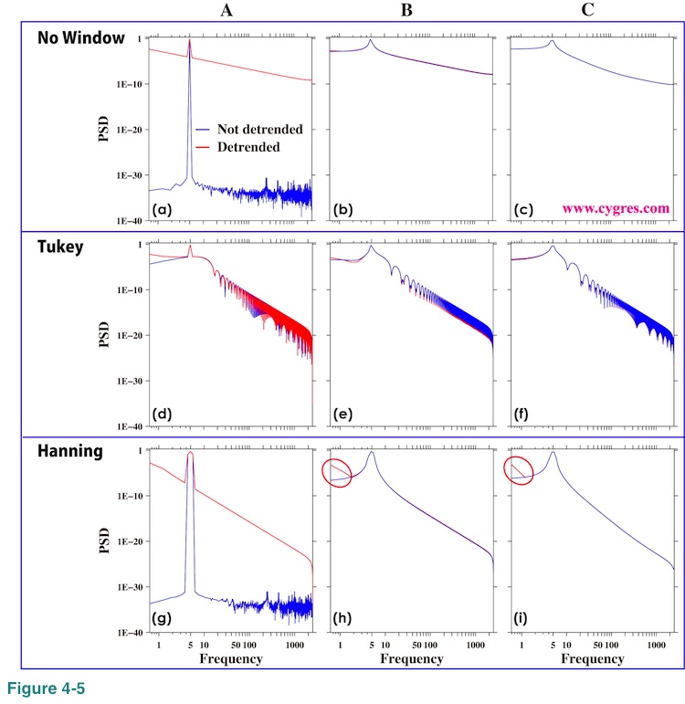
The cause of the difference we can see at the lowest frequency part of PSD when data length is B or C, marked by red circles in Figure 4-5(h) and (i), is slightly complicated. Figure 4-6(a), (b) and (c) show the same PSD as Figure 4-5(g), (h) and (i) except that we removed average from non-detrended data before computing PSD. PSD at the lowest non-zero frequency (left side edge of this graph) becomes larger than the PSD at one point right of it when data length is B or C (red circles; Figure 4-6 (b) and (c)). This is caused by removal of average before computing PSD combined with the effect of implicit FDS of Hanning window and this increase of PSD is artificial. We will show that implicit FDS of Hanning window occasionally un-smooth PSD in (4-2-7). Please remember that detrending also removes the average of the data.

We do not see similar behavior when we applied Tukey window with a default setting of 10% taper. This is because the weight of implicit FDS caused by Tukey window at a point next to the central point is much smaller than the one caused by Hanning window as shown by the fact that the width of peak is narrower (peak itself is sharper; Please see Figure 2-6). This fact causes the PSD, to which Tukey window is applied, at the lowest non-zero frequency not to be affected that much by value at zero frequency, which is practically zero because we removed the average.

Removing an average before computing PSD is often considered to be the minimum requirement to get a better estimate of PSD at a low frequency range if we do not detrend data. The reason behind it is that if we have a relatively large average and thus have a large PSD at zero frequency, PSD at lowest few bins are badly affected by zero frequency PSD because of implicit or explicit FDS. Thus, it may sound contradictory that we have artificially large PSD at the lowest non-zero frequency precisely because we removed average as we have shown here, this particular behavior is due to relatively rarely occurring un-smoothing effect of implicit FDS of Hanning window and, thus, it is not universal. Also, our test data is rather special and when we deal with real world data, we will have signals and noises at many frequencies and it will be rather rare to see an adverse effect of removing an average. Thus, we still recommend removing an average from data if we do not apply detrending.

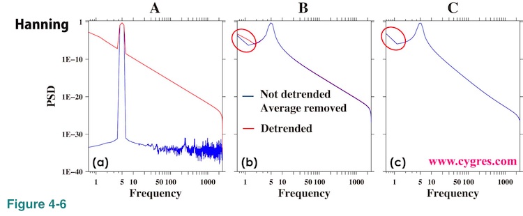
Figure 4-7(a) shows how the amplitude of signal bin varies as we add more data if we detrend data before computing PSD. Comparing this graph with Figure 2-4(b) (No detrending), we can see that amplitude of signal bin approaches to the actual signal amplitude much slower. This can be seen more clearly if we compare Figure 4-7(b) with Figure 2-4(c). Both of these graphs show amplitude of signal bin only at positions (asterisks) where frequency match occurs. Figure 4-7(c) shows that variance of data deviates considerably from theoretical variance of signal (0.5) when data length is shorter than 2.0 unlike variance shown in Figure 2-4(d). Although we can see these differences, the adverse effect on amplitude estimation of signal by PSD caused by detrending is relatively minor as long as data length is longer than a few periods of signal.

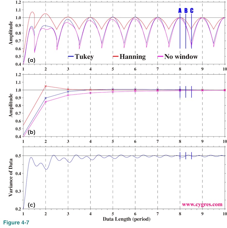
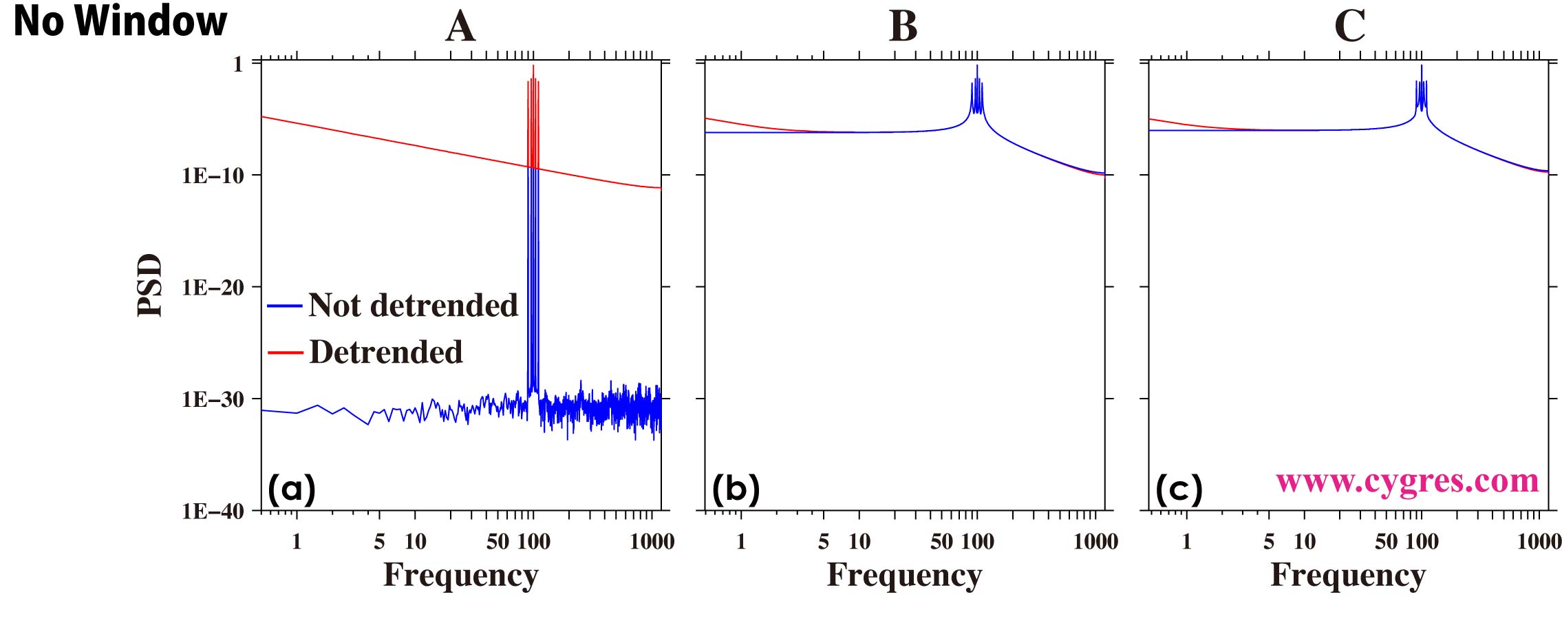
Figure 4-8 shows PSD when there are signals at multiple frequencies to demonstrate that the problem we described in this section is not limited to the case when we only have a single frequency signal. The data we used here is the noiseless data we used to compute PSD in Figure 2-22(red lines) and we did not apply any window function before computing PSD. In Figure 4-8(b) and (c) we can see that there are differences between detrended and non-detrended PSD at lower frequency range even when we have spectral leakage unlike previous example (Figure 4-5(b) and (c)). This is because effect of spectral leakage is relatively small at far left of these graphs simply because frequencies of those parts of graphs are far away enough from signal frequencies.

Now the question is what would happen if we have weak signals coexisting with a strong sinusoidal signal (Let us call it S1). To demonstrate this, we generated test data by adding part of data shown in Figure 1-1(a) to S1. In the following, let us call these added weak signals SR. Figure 4-9(a) shows time series of SR. We adjusted amplitude of SR so that the variance ratio of SR to S1 is 0.0001. The significant digit of our computation is large enough to keep SR faithfully. The unit of horizontal axis (Data Length) of this graph is not the same as Figure 1-1(a) but we chose this one for convenience. Figure 4-9(b) shows PSD of SR. We detrended SR and applied Tukey window before computing PSD. We made the unit of horizontal axis (Frequency) of this graph consistent with previous graphs. There are two peaks labeled S2 and S3 in this graph. We use these two peaks as targets to detect because variations represented by these peaks exist relatively steadily throughout the entire record of SR.

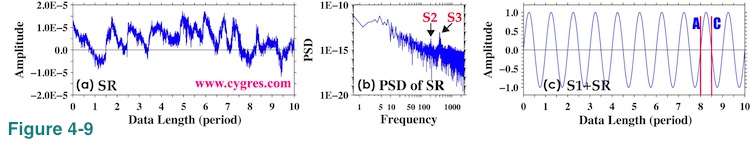
First, let us demonstrate when frequency of S1 is relatively low. The frequency of S1 is 5 cycles per 1 time unit of PSD (Data Length 5 is equivalent to 1 time unit) in this example. Figure 4-9(c) shows synthesized data, namely S1+SR. We cannot see SR in this graph at all because SR is much weaker than S1. In term of amplitude instead of variance, S1 is about 3 million (3.0E+6) times larger than S3. Please note that the range of vertical axis of Figure 4-9(c) is much larger than the range of vertical axis of Figure 4-9(a). We will show PSD when data lengths are A and C indicated by vertical red lines in Figure 4-9(c). Data length A is the case when frequency of S1 matches one of the frequencies of PSD and data length C is the case when difference between frequency of S1 and the nearest frequency of PSD (we called it frequency of signal bin before) becomes the largest as before. We omitted data length B to save some spaces.

Blue lines of upper three graphs of Figure 4-10 show PSD without detrending and without removing average when data length is A. This is the special case (we called it frequency match before) that we do not have spectral leakage of S1 at all. However, when we need to deal with real world data, it is quite likely that strong signal is composed of several different frequency components and it will be very difficult, if not impossible, to achieve frequency match like this. Therefore, we believe this case is good only for a demonstration. Having mentioned that, the blue and the red asterisks (*) in these graphs show the locations of S2 and S3. The black lines in Figure 4-10 show PSD of SR alone. For the sake of comparison, we did not detrend SR for these graphs and we moved these black lines downward to make comparison easier. The blue line in Figure 4-10(a) shows that PSD computation without detrending and without applying any window did do a superb job. It shows that the S1 affects PSD only at the frequency where S1 exists. When we applied Tukey window or Hanning window, Figure 4-10(b) and (c) show that PSD within a certain frequency range around S1 is dominated by S1 due to the implicit FDS and it is difficult to see PSD of SR within that frequency range.

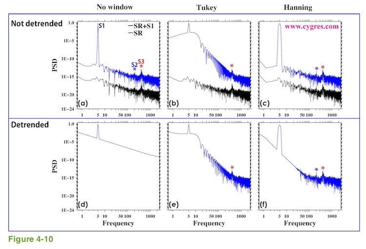
The lower three graphs of Figure 4-10 show PSD when we detrended data. Figure 4-10(d) shows that if we do not apply any window function, we are no longer able to see anything except S1 and the effect of added 'inclination' caused by detrending of S1. The reason why it is practically impossible to see PSD of SR if we detrend data is not that PSD of SR is buried under the PSD of the added 'inclination' generated by detrending (please see Figure 4-4(b)). PSD in this case is close to the summation of PSD of S1 and SR. There are two possibilities. The first one is truncation error. Showing the entire significant digits, PSD of the 'inclination' at the frequency of S3 is 0.1180623344177745E-9. There are 16 digits below decimal point. If PSD of S3 (Figure 4-9(b)) is less than 0.0000000000000001E-9 (15 zeros below decimal point), then adding PSD of S3 to the PSD of the 'inclination' would not change total PSD at all because of the limitation of the size of memory assigned to store that value. In our example this does not happen because the PSD at the peak of S3 is 0.00000681348403258001E-9 (5 zeros below decimal point). The second reason, and this is what happened here, is that the PSD of S3 is too small to make any detectable visual difference. Adding PSD of S3 to PSD of the 'inclination' would not change first 5 digits.

Figure 4-10(b) and (e) show that the difference between detrended and non-detrended PSD is relatively small when we applied Tukey window. The implicit FDS applied to S1 has a very strong influence on PSD across the wide frequency range and S2 is no longer detectable. We will describe more about this implicit FDS in the next section. We can see the hint of the effect of added 'inclination' at very low frequency range. If we applied Hanning window instead, detrended PSD (Figure 4-10(f)) shows a straight-sloped line at low frequency range caused by added 'inclination'. The effect of an implicit FDS is limited to one bin up and one bin down from the bin where S1 exists and we can get more information about SR than the case when we applied Tukey window.

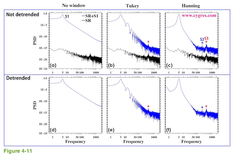
Figure 4-11 shows PSD when data length is C (Figure 4-9(c)) as an example when we have spectral leakage of S1 across the entire frequency range and this is more likely the case we would encounter. If we do not apply any window function (Figure 4-11(a) and (d)), the effect of spectral leakage overwhelms the effect of added 'inclination' as expected from Figure 4-5(c) and it is not possible to see anything except S1. Detrend or not does not make any practical differences. If we apply a window function, effect of spectral leakage is reduced but the effect of an implicit FDS is added and the difference between detrended and non-detrended PSD is difficult to see except at the lowest frequency. This difference at the lowest frequency is the same kind of difference we described using Figure 4-5 and Figure 4-6 (red circle). When frequency of S1 is higher we can clearly see the difference between detrended and non-detrended PSD especially when we applied a window function as we will show next.

Now, let us change the frequency of S1 and adjust data length accordingly, but keep anything else the same. Figure 4-12 shows PSD when data length is A. S1 is now located at 800. Again, PSD without applying any window function and without detrending is the best. S1 in Figure 4-12(a) appears to be sharper (width is narrower) than S1 in Figure 4-10(a) but this is only a result of visual effect caused by logarithmically scaled horizontal axis. If we compare Figure 4-12(d) with Figure 4-10(d), we can see that the PSD due to added 'inclination' becomes much smaller. This is expected from equation (17), which shows that PSD due to added 'inclination' is inversely proportional to the frequency of S1. We can even detect S2 (barely) and S3 in the detrended PSD. We will describe how the frequency of S1 affects detectability of SR in Appendix 4.

If we compare Figure 4-12(b) with Figure 4-10(b), we might think that effect of an implicit FDS when we applied Tukey window is considerably narrowed but, again, this is a result of visual effect of logarithmically scaled axis. The width and the magnitude of the effect of an implicit FDS do not depend on the frequency of S1.

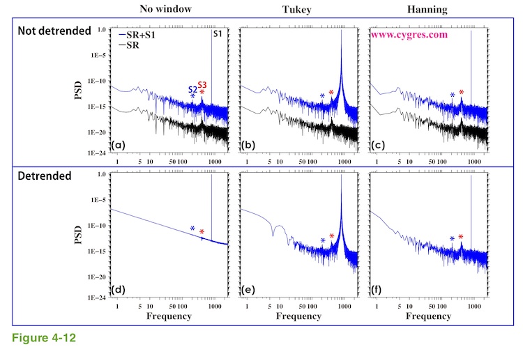
Figure 4-13 shows PSD when data length is C. If we do not apply any window function, we will miss SR completely. If we applied a window function, non-detrended PSD gives us more information about SR than detrended PSD does. Differences between non-detrended and detrended PSD are most prominent at low frequency range. When we applied Tukey window, SR deforms some of the typical bumps caused by S1 and it is slightly deceptive.

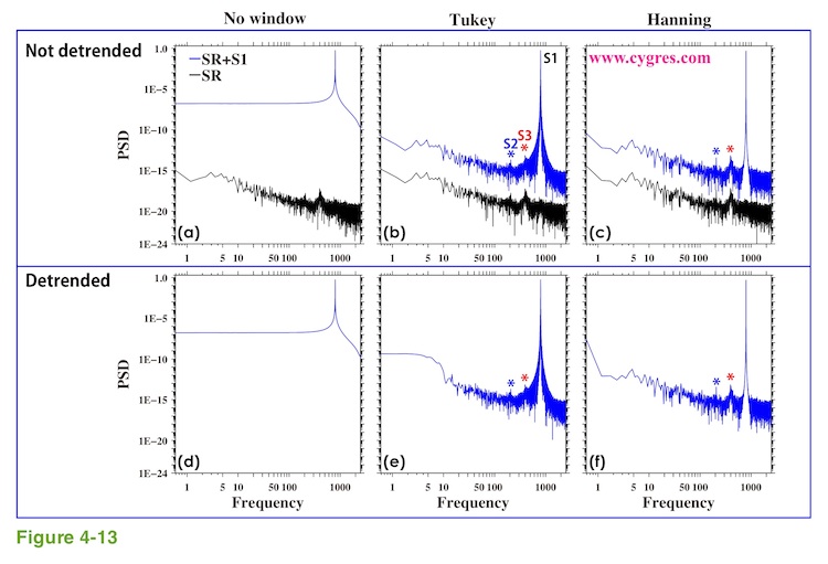
As a summary, if it is important to detect SR, these results suggest that using Hanning window without detrending might be the best choice although there are cases when Hanning window might cause a problem for a quite different reason as we will describe in (4-2-3).

However, if our data shows an obvious trend, we have to detrend data. The problem here is that the amplitude of S1 is too large compared with the amplitude of SR and ordinarily small effect of added 'inclination' due to detrending of S1 is enormous for SR. If amplitudes of most of the signals in SR are comparable to amplitude of S1, we will not see the effect of added 'inclination' just like blue lines of Figure 2-22. If our strong signals are limited within a relatively narrow frequency range, it might be better to apply a digital filter to our data in order to suppress strong signals before computing PSD. That method also reduces the effect of an implicit FDS and spectral leakage caused by strong signals. If our customers wish us to apply a filter before computing PSD, please, let us know. These results seem to show an awful effect of detrending but in reality we think the majority of us would never encounter data like this.

.

To read next page, please click right button below.