Power Spectral Density computation (Spectral Analysis)
MicroJob Package Deal Service PD001A/B(Copyright Cygnus Research International (Apr 20, 2015))

Page 4 of PD001A/B User Guide

Table of Content
(1) Summary of PD001A/B
(1-1) What this Package Deal service, PD001A does
(1-2) What PD001B does
(1-3) Summary of selectable computational parameters
(1-3-1) Detrending data (Applicable to all cases)
(1-3-2) Confidence interval percentage (Applicable to all cases)
(1-3-3) Taper ratio of a Tukey window (Applicable to cases B1, B2 and B3 only)
(1-3-4) FDS bin-width (Applicable to all cases except for cases A1, B1 and C1)
(1-4) Computational procedure
(1-5) Your Data (Input data)
(1-6) Products
(1-6-1) Data file (Product file)
(1-6-2) Graphs (Figures) in PDF (PD001A only)
(1-7) Price and ordering procedure
(1-8) Confidentiality
(2) Detail of the product
(2-1) Product files
(2-1-1) Format of Product file
(2-1-2) Explanation of contents of product files
(2-1-2-1) Frequency
(2-1-2-2) Period
(2-1-2-3) PSD
(2-1-2-4) Confidence interval of PSD
(2-1-2-5) Percent of variance
(2-1-2-6) Amplitude (Amplitude spectrum)
(2-1-2-7) Phase
(2-1-3) How to use/interpret data in our product file
(2-1-3-1) Drawing graphs
(2-1-3-2) PSD and Confidence interval of PSD
(2-1-3-3) Estimating amplitude of variations at specific frequencies using amplitude spectrum
(Case 1) When the signal is a sinusoid and the amplitude of it is constant or almost constant in time
(Case 2) When the signal itself is not a sinusoid but the composition of sinusoids of various frequencies
(Case 3) When the signal is sinusoid but the amplitude of the signal varies in time
(Case 3-1) Variation of amplitude itself is sinusoidal
(Example 1) Amplitude of sinusoidal oscillation of frequency f0 varies sinusoidally.  Frequency of amplitude variation is f1 and f1 is smaller than f0. Both f0 and f1 are constants.
(Example 2) Amplitude of sinusoidal oscillation of frequency f0 is summation of a constant and a sinusoidal variation of frequency f1.
(Case3-2) Amplitude of sinusoidal oscillation of frequency f0 varies but that variation does not resemble to a sinusoid.
(Case4) When the signal is periodic but the signal does not look like a sinusoid
(2-1-3-4) Obtain some idea how strong the variations within a specific frequency range are.
(2-1-3-5) Construct digitally filtered time series data
(2-1-3-6) Alternative method of amplitude estimation
(2-2) Graph
(3) How to prepare data for this package
(4) Guide for setting proper selectable parameters
(4-1) Detrending and removing average; Yes or No? Default setting is Yes.
(4-1-1) What is detrending? Why do we have to do that?
(4-1-2) Example of detrending
(4-1-3) When detrending becomes harmful
(4-2) Taper ratio of Tukey window; 0~100(%) Default setting is 10%
(4-2-1) Why we need to apply a window function
(4-2-2) What does window function do
(4-2-3) Why Hanning window is not necessarily a good solution
(4-2-4) Why we provide non-windowed and Tukey windowed result for PD001A
(4-2-5) The method to reduce dumping near the both ends of data while still using Hanning window
(4-2-6) Implicit FDS
(4-2-7) Implicit FD'Smoothing' Really?
(4-2-8) Reduction of PSD and amplitude due to the window
(4-2-9) Does correction of reduction of PSD work well?
(4-2-10) Tukey window; how taper ratio affects its characteristics
(4-3) Bin-width of FDS; 1,3,5,7,... (Odd integer); Default setting is None, 3 and 7
(4-3-1) FDS works well for PSD
(4-3-2) FDS does NOT work well for amplitude spectrum
(4-3-3) Frequency resolution when we applied FDS
(4-3-4) Alternative method of FDS
(4-4) Percentage of confidence interval; any positive value larger than 0.0 and smaller than 100.0; Default is 95.0

Appendix 1; About numerical error generated by computers.
Appendix 2; Spectral leakage of power spectrum density function and window functions.
Appendix 3; Why we see a single peak instead of twin-peaks when data length is short.
Appendix 4; How the frequency of S1 affects the detectability of SR

One of the ways to compare S' with S is comparing outline, usually called envelope, of S' with envelope of S. Figure 2-29 shows part of S in Figure 2-19 and its upper side envelope. This upper side envelope is equal to (please see equation (7))

Lower side envelope is just a mirror image of upper side envelope. In case of an AM radio signal, this envelope is the real meat, containing voices and music, and some radio transmitters only transmit one side of envelope. There may be cases when we want to analyze variations of amplitude of a signal propagated through a medium in order to know the internal variations of physical characteristic of that medium. We prpbably want to see envelope in those cases.

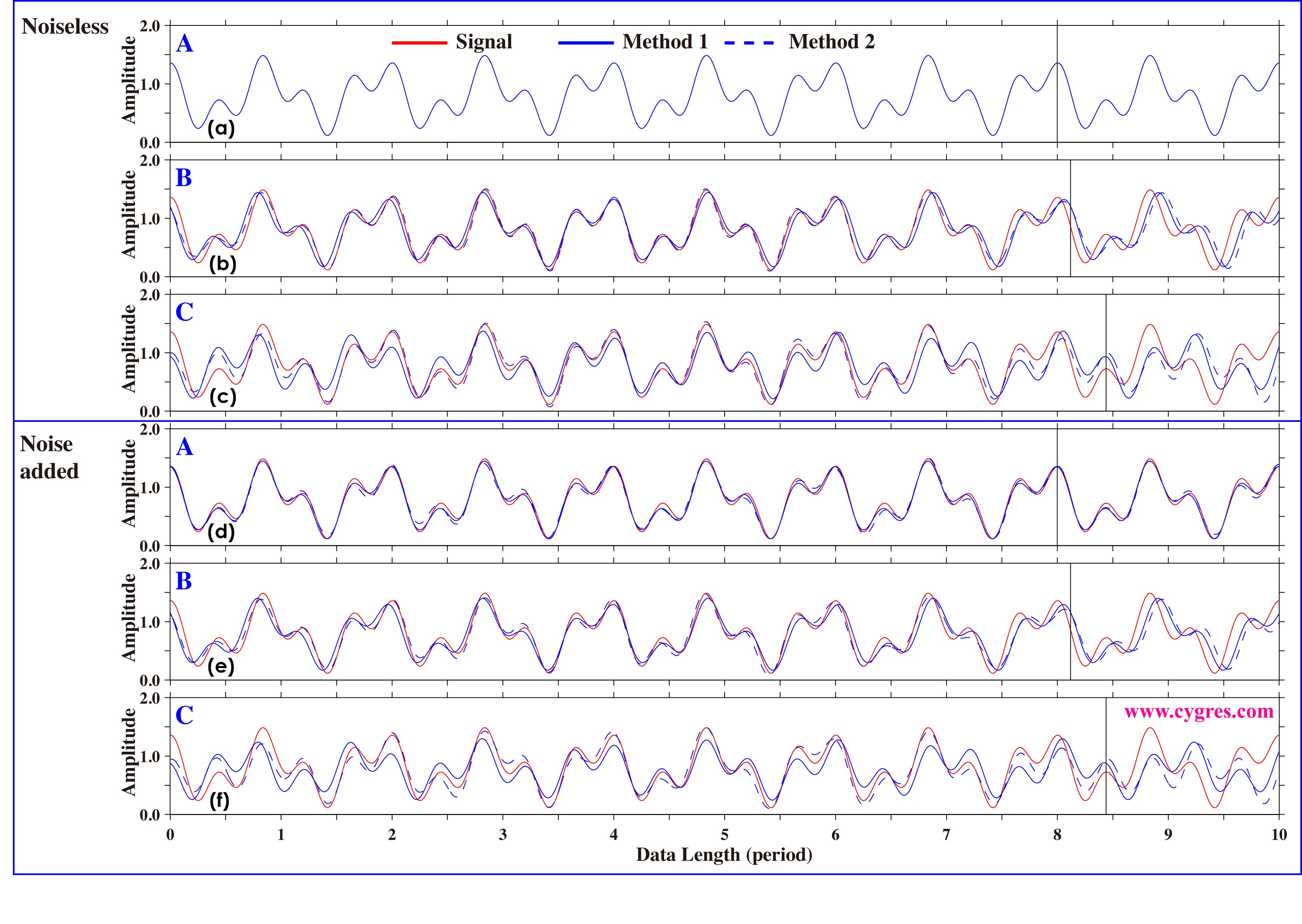
Since our computed amplitude of V1 is not equal to that of V2 and computed amplitude of V3 is not equal to that of V4 as shown in Figure 2-24, in the strict sense, we cannot apply AM radio signal analogy to our computational result. Nevertheless, it provides easier way to see how much our reconstructed signal S' differs from actual signal S.

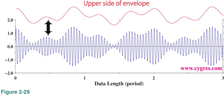
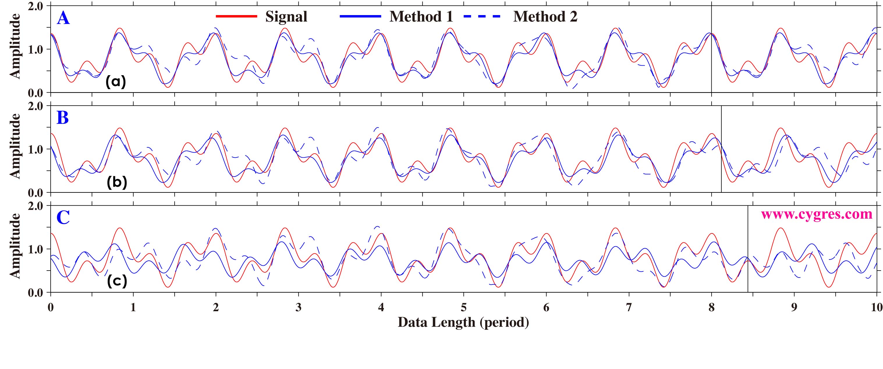
Figure 2-30 shows upper side envelopes of S (red solid line), S' by the Method 1 (blue solid line) and S' by the Method 2 (blue dashed line). Upper three graphs are the results when we used noiseless data S and lower three graphs are the results when we used noise added data. We can only see a blue solid line in Figure 2-30(a) but this is because S and S' are practically identical in this case. These graphs suggest that (a) addition of noise of this magnitude does not affect accuracy of reproduced signal (S') that much, (b) accuracy of reproduced signal becomes best in the middle of data but degrades near the both end of data and (c) mismatch of actual signal frequencies and frequencies of signal bins does cause relatively large error of signal reproduction. The reason of (b) is as follows. f1 and f2 in equation (11) of S' differ from those of S if frequencies of signal bins differ from actual signal frequencies. Then if envelope of S' matches envelop of S fairly well at position X, discrepancy between them tends to grow as we move away from X. In our case, X is located at the middle point of data used for amplitude spectrum computation (portion of time series left of vertical black lines). Noise is not the direct cause of this phenomenon.

Now, let us make noise three times larger than previous example. Figure 2-31(a) shows time series of signal (S; red), noise (N; purple) and data (S+N; blue) in this case. The signal is the same as before and the reason why S in Figure 2-31 looks smaller than S in Figure 2-19(a) is because we changed vertical scale of the graphs. Figure 2-31(b) shows expanded view of S and data. The standard deviation of noise is about 3.00 and it is difficult to see S in Data in Figure 2-31(b) unlike in the previous example (Figure 2-19(b)).

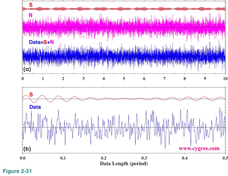
Figure 2-32 shows how amplitudes and phases of signal bins vary as we add more data. If we compare these graphs with Figure 2-20, we can see that the amplitudes of signal bins deviate much more from their respective actual signal amplitudes (horizontal black lines in Figure 2-32 (a) and (b)) this time. These graphs suggest that a large amount of data is necessary to get fairly accurate signal amplitudes. Although we have chosen the same data lengths (A, B and C in Figure 2-32 (a) and (c)) for detailed inspections described below for the sake of consistency, those data lengths are likely too short to get relatively accurate signal amplitudes and phases this time.

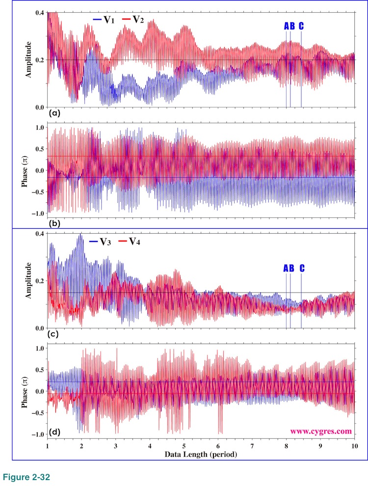
Figure 2-33 shows amplitude spectra. Data lengths for these computations are the same as before and indicated in Figure 2-32(a) and (c) (vertical solid blue lines labeled A, B and C). One of the important differences between these spectra and those shown in Figure 2-24 is that peaks generated by noise are as large as signal peaks. In other words signal peaks are no longer easily identifiable. If we do not have prior knowledge of signal frequencies, we will miss most of them in this example. As to the accuracy of amplitude relative to those of previous example, it is somewhat a mixed bag.

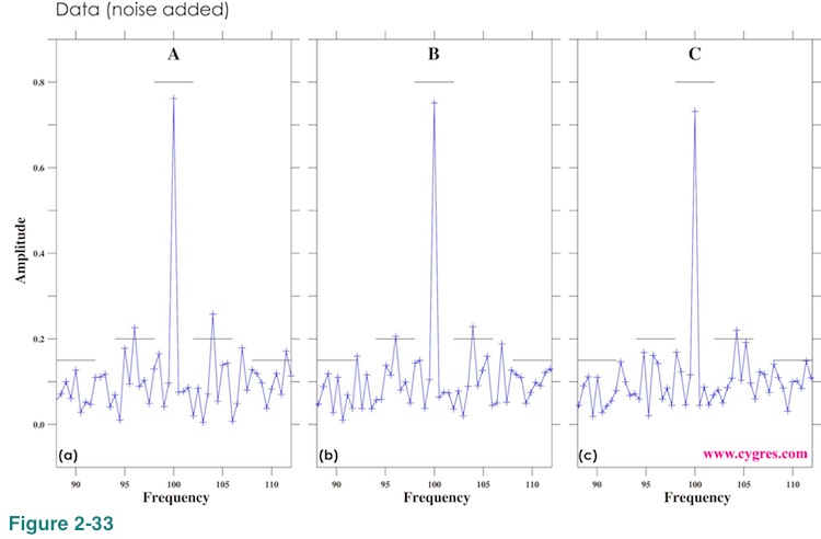
Figure 2-34 shows upper side envelopes of reproduced signals (S') as before. We omit S' using noiseless data in this graph because they are the same as before (Figure 2-30). Considering that the amplitude of noise relative to signal in this example is very large, we feel that reproduction of signal by these methods does fairy good job but this is just our subjective opinion. Probably the real problem in this example is that it is very difficult to know which peaks in amplitude spectrum are due to signal and which peaks are due to noise (Figure 2-33).

(2-1-3-6) Alternative method of amplitude estimation
Finally, we briefly explain an alternative method of amplitude estimation although we will not add computation based on this method in this package deal service since computational procedure of this method is quite different from PSD computation. If there are enough demands we will make another package deal service, which uses this method in the future.

To apply this method we need to know exact signal frequencies but we do not need to care about frequency match. Also, this method does not demand constant sampling interval. The results we show below make us feel this method is more convenient than PSD computation for amplitude estimation. However, this method has several disadvantages. The accuracy of the result of this method critically depends on the accuracy of the knowledge of signal frequencies. It would take too much time to compute amplitudes of thousands of frequencies.

The method we show here tries to approximate data as summation of signals and error where error does not correlate with any of the signals.  This can be expressed as

In this equation "Data" and frequencies of signals (Fm) are given and we evaluate amplitudes (Hm) and phases (Qm). "Error" is initially unknown and will be computed by this method but it is a sort of by-product and we usually do not use it. The important thing to be noted here is that Um in this equation is NOT equal to Vm in equation (10) and "Error" in this equation is NOT equal to "Noise" in equation (10). Equation (12) shows the relationship between "Data" and result of statistical computation applied to "Data" while equation (10) shows construction of "Data". These two equations are fundamentally different. We generated "Noise" in equation (10) using random number generator. The correlation between this "Noise" and V0, V1, V2, V3 or V4 is very low and we ordinarily say that "Noise" is not statistically correlated with any of Vms but that does not mean correlation coefficients between them are all zero. The method we describe here makes correlation coefficients between "Error" and U0, U1, U2, U3 or U4 in equation (12) zero within computational accuracy.

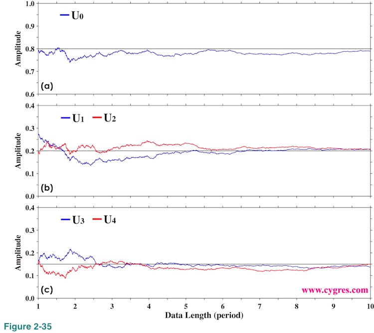
Figure 2-35 shows how computed amplitudes of U0, U1, U2, U3 and U4 vary as we add more data when we use data shown in Figure 2-19. The horizontal black solid lines in these graphs show actual signal amplitudes. These graphs show that computed amplitudes do not oscillate like those shown in Figure 2-20. This is what we mean by "we do not need to care about frequency match". If we ignore those oscillations in Figure 2-20 we can probably see the patterns common to both Figure 2-20 and Figure 2-35. These graphs might make us think PSD computation is far inferior to this method, but we should not forget that the primary purpose of computing PSD is usually to find signal frequencies. We can use this method only if we know signal frequencies beforehand.

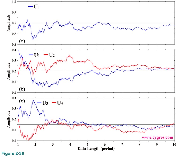
When we use the data shown in Figure 2-31, computed amplitudes differ more from actual signal amplitudes as shown in Figure 2-36.

(2-2) Graph
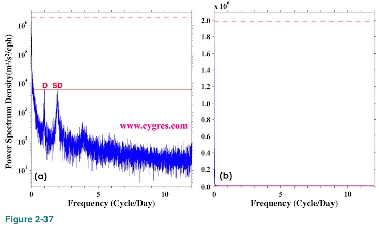
We provide graphs of PSD in a PDF format if you order PD001A (No graphs for PD001B). We use logarithmic scaling for vertical axis and linear scaling for horizontal axis. The variable for horizontal axis is frequency instead of period. Logarithmic scaling visually expands low value range while compresses high value range. We have chosen logarithmic scaling for vertical axis as commonly done because magnitude of the variation of PSD is quite large in many cases. Figure 2-37(a) shows an example of PSD with logarithmically scaled vertical axis and linearly scaled horizontal axis. PSD shown in this graph is the same as PSD shown in Figure 1-1(b) where we used logarithmically scaled horizontal axis. As mentioned before, PSD is computed at frequencies with constant interval. Therefore, interval of horizontal position (frequency) where PSD is computed is constant in Figure 2-37(a). The red horizontal solid line in this graph shows value of PSD at D and the red horizontal dashed line shows the maximum value of PSD. Although the visual vertical distance between these two lines is less than half of the height of this graph, the maximum value of PSD is more than 313 times larger than the value of PSD at D. Therefore, if we use lineally scaled vertical axis as in Figure 2-37(b), it will be practically impossible to find peaks at D. As a matter of fact, it is very difficult to see anything other than the red horizontal dashed line in Figure 2-37(b). The horizontal axis at bottom is red because horizontal solid line indicating value of PSD at D is there. If we are interested in PSD at lower frequency range rather than at higher frequency range it might be useful to use logarithmically scaled horizontal axis.

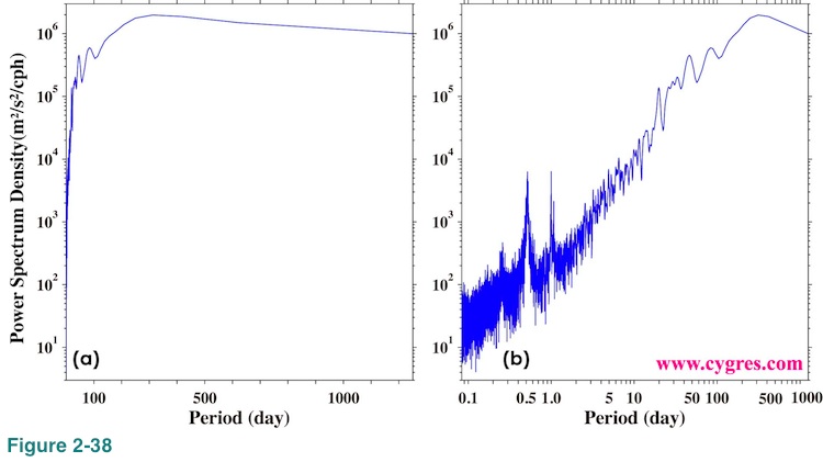
It is possible to use period instead of frequency for horizontal axis. In that case lineally scaled horizontal axis, Figure 2-38(a), will produce somewhat useless graph unlike Figure 2-37(a). The longest period in this example is 1250 days if we exclude the one whose period is infinite (Frequency is zero). While there are 14988 bins whose periods are shorter than 100 days, there are only 13 bins whose periods are longer than 100 days. This is because period is the inverse of frequency. In Figure 2-37(b) we used logarithmic scaling for horizontal axis.

If there are strong demands we may make axis scaling selectable in the future but at this time, we make graphs with logarithmic scaling for vertical axis, linear scaling for horizontal axis and frequency for horizontal axis similar to Figure 2-37(a).

(3) How to prepare data for this package
In this section we briefly describe how to make a data file for PD001A and PD001B from an Excel file. If you wish us to compute PSD of more than one data set with different data length (number of data) unlike example shown below, please create multiple files so that the data length of variable(s) contained in each file is the same. For example, let's assume you wish us to compute PSD of variables A, B and C and the data lengths of those are 20, 30 and 20. Then, please create one file, which contains variable A and C, and create another file, which contains variable B alone. Alternatively, creating three files, each of which contains single variable, will also be fine.

Step 1: Open target Excel file.

Step 2: Select cells you wish us to process.
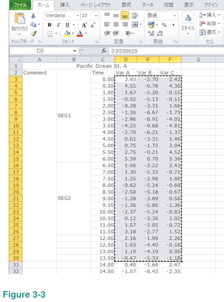
Let's say you wish us to compute PSD of Var A and Var C but use only those between row number 3 and row number 30 in the example shown below. (Please ignore menu language.) Now, select the cell of the upper left corner of the data segment as shown below (column D, row 3).

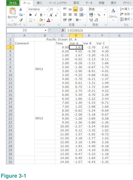
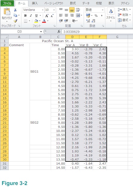
Then drag cursor all the way to the bottom right cell of the data segment (column F, row 30) while keep pressing right button of your mouse.

Please, make sure your selection contains only numbers. The selected area above contains Var B (you wish us to compute PSD of Var A and Var C but not Var B) but that will not be a problem.

Step 3: Copy data.
This is a standard copy and paste (Step5) procedure. Either pressing CTRL+C or right clicking and selecting "copy" would do this.

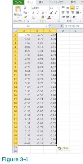
Step 4: Open new work sheet.

Step 5: Paste what you have copied in a new work sheet.
Result will look like below. It still contains Var B data but that will be fine. If you prefer, you can delete them by deleting column B. Please note that this new work sheet contains only numbers but nothing else. It also does not have any merged cells.

Step 6: Save this new work sheet as a "CSV (Comma delimited)" file.

Step 7: Make a note about which column(s) is(are) data you wish us to process. (Optional)
In this example columns A and C are the ones you wish us to compute PSD. It is not necessary to remove column B as long as you notify us which columns are to be processed.

If you open saved file using Microsoft's Notepad application, it looks like below.

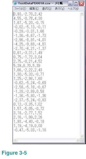
You may have noticed that the positions of commas are not aligned vertically but that is fine. Only the important things are that number of data is the same for all row/line (in this example there are 3 data per row) and data are separated by a single comma between them.

To read next page, please click right button below.