Page 6 of PD001A/B User Guide

Table of Content
(1) Summary of PD001A/B
(1-1) What this Package Deal service, PD001A does
(1-2) What PD001B does
(1-3) Summary of selectable computational parameters
(1-3-1) Detrending data (Applicable to all cases)
(1-3-2) Confidence interval percentage (Applicable to all cases)
(1-3-3) Taper ratio of a Tukey window (Applicable to cases B1, B2 and B3 only)
(1-3-4) FDS bin-width (Applicable to all cases except for cases A1, B1 and C1)
(1-4) Computational procedure
(1-5) Your Data (Input data)
(1-6) Products
(1-6-1) Data file (Product file)
(1-6-2) Graphs (Figures) in PDF (PD001A only)
(1-7) Price and ordering procedure
(1-8) Confidentiality
(2) Detail of the product
(2-1) Product files
(2-1-1) Format of Product file
(2-1-2) Explanation of contents of product files
(2-1-2-1) Frequency
(2-1-2-2) Period
(2-1-2-3) PSD
(2-1-2-4) Confidence interval of PSD
(2-1-2-5) Percent of variance
(2-1-2-6) Amplitude (Amplitude spectrum)
(2-1-2-7) Phase
(2-1-3) How to use/interpret data in our product file
(2-1-3-1) Drawing graphs
(2-1-3-2) PSD and Confidence interval of PSD
(2-1-3-3) Estimating amplitude of variations at specific frequencies using amplitude spectrum
(Case 1) When the signal is a sinusoid and the amplitude of it is constant or almost constant in time
(Case 2) When the signal itself is not a sinusoid but the composition of sinusoids of various frequencies
(Case 3) When the signal is sinusoid but the amplitude of the signal varies in time
(Case 3-1) Variation of amplitude itself is sinusoidal
(Example 1) Amplitude of sinusoidal oscillation of frequency f0 varies sinusoidally.  Frequency of amplitude variation is f1 and f1 is smaller than f0. Both f0 and f1 are constants.
(Example 2) Amplitude of sinusoidal oscillation of frequency f0 is summation of a constant and a sinusoidal variation of frequency f1.
(Case3-2) Amplitude of sinusoidal oscillation of frequency f0 varies but that variation does not resemble to a sinusoid.
(Case4) When the signal is periodic but the signal does not look like a sinusoid
(2-1-3-4) Obtain some idea how strong the variations within a specific frequency range are.
(2-1-3-5) Construct digitally filtered time series data
(2-1-3-6) Alternative method of amplitude estimation
(2-2) Graph
(3) How to prepare data for this package
(4) Guide for setting proper selectable parameters
(4-1) Detrending and removing average; Yes or No? Default setting is Yes.
(4-1-1) What is detrending? Why do we have to do that?
(4-1-2) Example of detrending
(4-1-3) When detrending becomes harmful
(4-2) Taper ratio of Tukey window; 0~100(%) Default setting is 10%
(4-2-1) Why we need to apply a window function
(4-2-2) What does window function do
(4-2-3) Why Hanning window is not necessarily a good solution
(4-2-4) Why we provide non-windowed and Tukey windowed result for PD001A
(4-2-5) The method to reduce dumping near the both ends of data while still using Hanning window
(4-2-6) Implicit FDS
(4-2-7) Implicit FD'Smoothing' Really?
(4-2-8) Reduction of PSD and amplitude due to the window
(4-2-9) Does correction of reduction of PSD work well?
(4-2-10) Tukey window; how taper ratio affects its characteristics
(4-3) Bin-width of FDS; 1,3,5,7,... (Odd integer); Default setting is None, 3 and 7
(4-3-1) FDS works well for PSD
(4-3-2) FDS does NOT work well for amplitude spectrum
(4-3-3) Frequency resolution when we applied FDS
(4-3-4) Alternative method of FDS
(4-4) Percentage of confidence interval; any positive value larger than 0.0 and smaller than 100.0; Default is 95.0

Appendix 1; About numerical error generated by computers.
Appendix 2; Spectral leakage of power spectrum density function and window functions.
Appendix 3; Why we see a single peak instead of twin-peaks when data length is short.
Appendix 4; How the frequency of S1 affects the detectability of SR

(4-2) Taper ratio of Tukey window; 0~100(%) Default setting is 10%
In the following, we first explain a general concept of window functions and then we will show some details about a Hanning window function before showing how changing taper ratio of a Tukey window function would affect PSD computation. This is because the characteristic of a Tukey window function varies from the one equivalent to that of non-window by selecting taper ratio of 0% to the one equivalent to that of a Hanning window function by selecting taper ratio of 100%. We will describe some other details of window functions not particularly related to selectable parameters of this package deal service but we hope those descriptions will help our customers interpreting the contents of our product file. In this section we occasionally use a word 'window' as a verb.  For example, 'Hanning windowed PSD' means PSD of data to which a Hanning window function is applied.

(4-2-1) Why we need to apply a window function
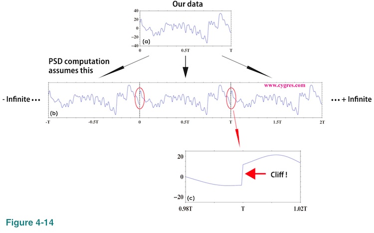
When we compute PSD by a commonly used method, which we also use in this package deal service, we implicitly assume that the data we have (Figure 4-14(a)) is just a segment of infinitely long data in which our data repeats itself infinitely as shown in Figure 4-14(b). The frequencies we compute PSD are consistent with this assumption.

This assumption connects the end point of our data to the start point of our data as shown in red ellipses in Figure 4-14(b) and if there is a 'cliff' caused by the difference of values at the end point and the start point of data as shown in Figure 4-14(c), it will raise PSD across entire frequency range. The purpose of applying a window function is to remove these cliffs so that this artificial increase of PSD would be reduced. This artificial increase of PSD is spectral leakage and we will describe more about the relationship between spectral leakage and window functions in Appendix 2.

(4-2-2) What does window function do
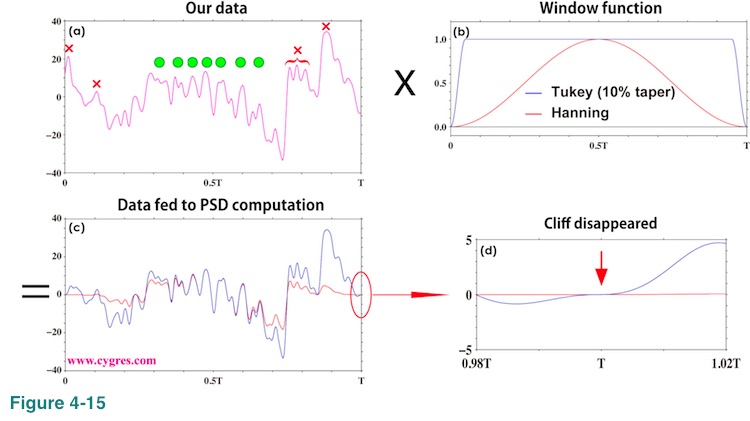
Applying a window function or, simply, windowing means that we multiply our data (Figure 4-15(a)) by a window function (Figure 4-15(b)). The resultant data (Figure 4-15(c)) is the actual data PSD computation uses and Figure 4-15(d) shows that this process removes 'cliff' at boundaries. Please note that the vertical scales of figures 4-15(c) and (d) are different. The last value (value at the rightmost point in the graph) of a window function is always 0.0.

(4-2-3) Why Hanning window is not necessarily a good solution
One of the aspects of data shown in Figure 4-15(a) is that the characteristics of variation vary a lot depending on where we look at. This particular aspect makes usage of commonly recommended Hanning window not necessarily attractive. In case of Hanning window, the value of window function is less than 0.5 for half of the entire length (Figure 4-15(b)). Combined with these two factors, relatively stable periodic variations in the middle of original data indicated by green circles in Figure 4-15(a) are well preserved in Figure 4-15(c) (red line) but some noticeable features near the both ends of data indicated by red crosses are heavily dumped in Figure 4-15(c). The data shown here is not an artificially created data for a demonstration but a short segment of real data shown in Figure 1-1(a). We applied a band pass filter to remove very low and high frequency components of data. Otherwise our data would look like a very spiky (high frequency components) slow variation (low frequency components) and those features marked by green circles in the graph will be obscured.

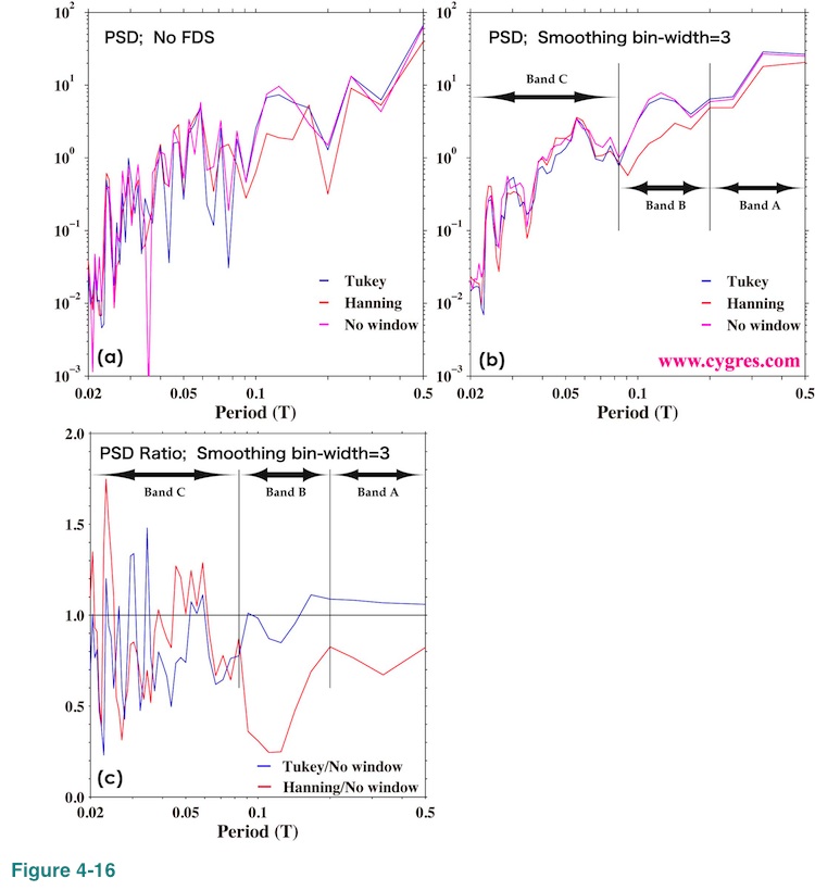
Figure 4-16(a) shows PSD of this data with and without windowing.  Since this graph is too complicated to make comparisons, we applied 3-bin FDS and the results are shown in Figure 4-16(b).  This graph shows that the Hanning windowed PSD is consistently smaller than the others within Band B, and, to the lesser degree, within Band A.  Hanning windowed PSD divided by non-windowed PSD shown in Figure 4-16(c) indicates this feature more clearly.

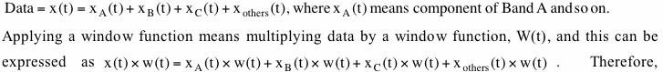
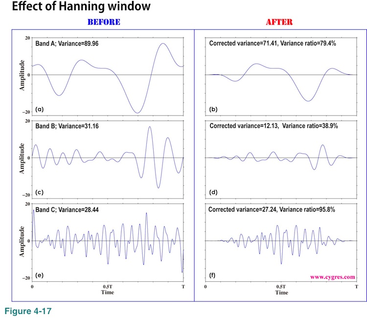
The left part of Figure 4-17 ((a), (c) and (e)) shows filtered time series for bands A, B and C computed by the method described in (2-1-3-5) using non-windowed amplitude spectrum and the right part of Figure 4-17 ((b),(d) and (f)) shows the result of windowing for each of these components. By using equation (3), we can express our data as a summation of 4 components each covering different frequency range as

inspecting these graphs will help us getting an idea why Hanning windowed PSD shows smaller values within Band B but not within Band C. One of the quantities to represent magnitude of these variations is the variance and we show them in these graphs. 'Corrected variance' in right side panels means that we corrected variance of windowed time series using commonly used method for windowed PSD (Please see (4-2-8)) so that we can compare these values in the right panels directly with 'Variance' in the left panels. This correction does not depend on frequency. The 'Variance ratio' is 'Corrected variance' of windowed time series (right side panels) divided by 'Variance' of un-windowed time series (left side panels). This ratio roughly shows how much of variation is lost by applying Hanning window. Figure 4-17(c) shows that large variations within Band B exist mostly near the both ends of time series and Figure 4-17(d) shows that Hanning window significantly dumps them. This dumping makes Hanning windowed PSD significantly smaller than non-windowed PSD in this frequency range. To the lesser degree, the same can be said to Band A. On the other hand, Figure 4-17(e) shows that the amplitude of variations in Band C is relatively uniform throughout the entire time series. As a result, reduction rate in this frequency range is very small and the difference between Hanning windowed and non-windowed PSD is relatively small.

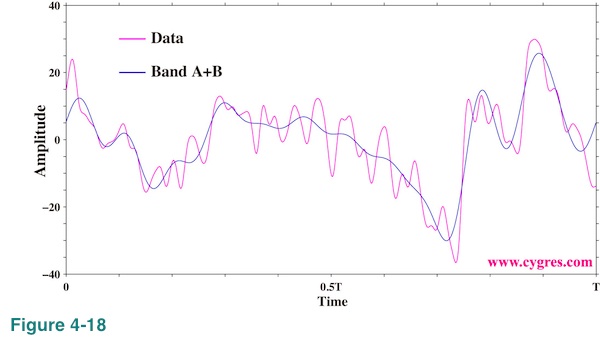
This is not really important for the argument here, but summation of bands A and B reproduces approximate profile of data as shown in Figure 4-18. Therefore, Band A and Band B are very important in this particular case.

(4-2-4) Why we provide non-windowed and Tukey windowed result for PD001A
When we need to deal with industrial or engineering data in which signals are generated by more or less regulated engines, motors and oscillators, we can expect that statistical characteristics of data do not change that much from one moment to another. Then, it does make sense to think that strong dumping of data near both ends caused by Hanning window would not make any serious problem in those cases. However, when we analyze data of natural sciences or human activities (stock price, for example), statistical characteristics might change a lot from one moment to another as in the case we have shown here. For this reason we provide non-windowed and Tukey windowed PSD as well as commonly recommended Hanning windowed PSD if our customer order PD001A so that our customers can chose the best result among them. There are many other window functions and choosing the best one among them is rather a mind-boggling task. Our strategy here is, 'Let's compute them all first and think about a window later!'.

(4-2-5) The method to reduce dumping near the both ends of data while still using Hanning window (Not supported in this package deal service)

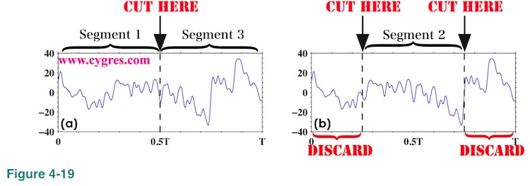
One of the methods to reduce dumping near the both ends of data while still using Hanning window is to use so called Welch's method. At this moment we do not have an intention to implement this method in this package deal service but we describe it briefly here.

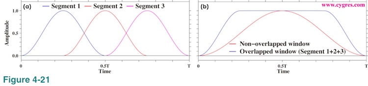
First, we cut the data in the middle along the dashed line in Figure 4-19(a). This will produce two data segments. Then we chop off the data along the dashed lines in Figure 4-19(b) and pick up the central part of the data.

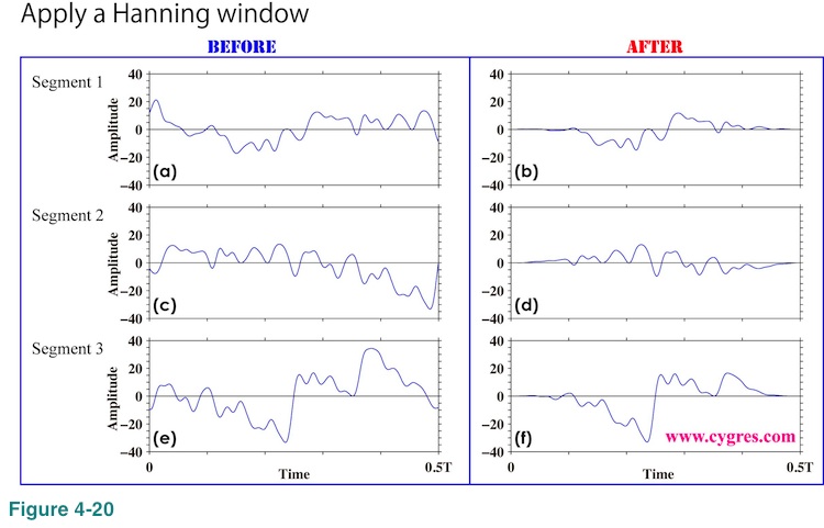
Now we have three data segments of equal length. Then, we apply Hanning window to each of these data segments individually as shown in Figure 4-20 and compute PSD of each. This will give us three sets of PSD.

After that, we compute average of PSD for each bin (ensemble average) from these three sets of PSD. Figure 4-21(a) shows the weight, which is a value of a Hanning window function, multiplied to data. This graph also shows the coverage of individual data segment. The trick is that by allowing overlapping of data segments in this way, we can reduce the portion where excessive dumping occurs. If we add three curves in Figure 4-21(a) together we will get 'Overlapped window' in Figure 4-21(b) (blue line). The red line in this graph is the weight of an ordinary (non-overlapped) Hanning window function for a comparison. When we use Welch's method, some values of data are used more than once. Half of the data are used twice in this example.

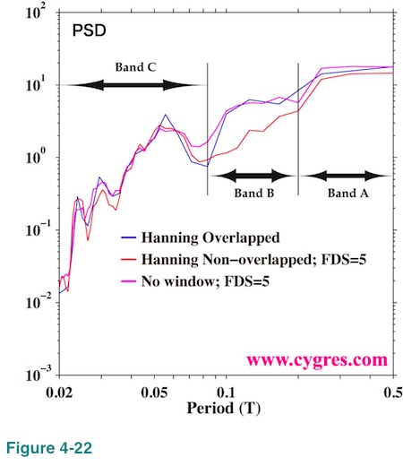
The blue line in Figure 4-22 shows PSD computed by this method and the purple line in this graph shows non-windowed PSD. We applied 5-bin FDS to the non-windowed PSD to make comparison easier. The reason why we specifically choose 5-bin for FDS bin-width here is as follows. Firstly, the data length of individual data segment when we applied Welch's method is half of original data length. Then, frequency width of each bin is twice as wide as frequency width of each bin when we did not apply Welch's method. Secondly, the width of implicit FDS caused by Hanning window is three-bin as we will explain in (4-2-6). Since we cannot chose even number for the bin-width of explicit FDS, we decided to have 5-bin instead of 6-bin for FDS bin-width.

The red line in this graph shows non-overlapped (ordinary) Hanning windowed PSD. The purple and the red lines are the same as those in Figure 4-16(b) except for the bin-width of FDS. This graph shows that the reductions of PSD within bands A and B are considerably reduced if we use Welch's method. Thus, we can conclude that the reductions of PSD within bands A and B when we applied ordinary Hanning window are artificial and Welch's method will fix a problem. However, there is a price to pay; the frequency resolution is worsened and the lowest non-zero frequency of PSD (third raw of our data file) increases since the data length of each segment is shorter than the original data.

(4-2-6) Implicit FDS
Another effect of applying a window function to data is implicit FDS. This implicit FDS is automatically integrated at the point when data is multiplied by a window function unlike explicit FDS we apply later in the computation. We use mathematics relatively heavily in this section to explain this topic since we have not found any way to explain how this thing works without using equations. Again, if you are considering placing an order we will be happy to answer your questions.

First of all, one-sided windowed continuous PSD is the square of absolute value of Fourier transform of data multiplied by a window function divided by length (time) of data and multiplied by 2. This is very mouthful but if we use a pseudo equation, it can be expressed as

The Fourier transform generally produces so called complex numbers that consist of a real part and an imaginary part. The absolute value means square root of square of a real part plus square of an imaginary part.

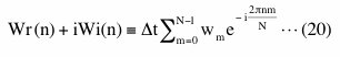
Instead of using a continuous form of Fourier transform to compute continuous PSD, we usually use a discrete form of Fourier transform to compute PSD at discrete frequencies. The discrete Fourier transform of data, xm where the subscript m is the index ranging from 0 to N-1, at the frequency of k_th (k is 0 to N/2 where N is the number of data) bin is

The subscripts r and i in the left hand side of equation (18) stand for a real part and an imaginary part of a complex value, respectively. Then, non-windowed PSD of k_th bin is

Now, Fourier transform of data xm multiplied by a window function wm is the convolution of the Fourier transform of xm and the Fourier transform of wm according to the Convolution theorem. The important point here is that this convolution of the Fourier transform of xm and the Fourier transform of wm is the same as a moving average of the Fourier transform of xm with the non-uniform weights which are the Fourier transform of wm except that the summation of weights is not equal to 1.0. Let Fourier transform of a window function wm at the frequency of n_th bin be

Here we intentionally use 'n' instead of 'k' as an index because we want to use Wr(n) and Wi(n) as weights in the convolution we will do later. In case of Hanning window, Wr(0)=T/2, Wr(1)=Wr(-1)= - T/4 but others are all zero.

Using Convolution theorem, equation (18), equation (20) and the fact that all the Wr(n) and Wi(n) except for Wr(0), Wr(1) and Wr(-1) in equation (20) are zero, Fourier transform of data multiplied by a Hanning window function at the frequency of k_th bin can be expressed as

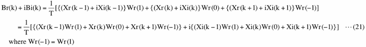
The coefficient 1/T in the right hand side of above equation is equal to the frequency width of bins. When k is 0, we replace k-1 with N/2 and when k is N/2, we replace k+1 with 0. Using the fact that Wr(-1)=Wr(1)= - T/4 and Wr(0)=T/2, equation (21) can be simplified as

If we consider "Wr" as weights, the right hand side of equation (22) is simple 3-point weighted moving average (again, in the strict sense it is not an average because the summation of weights is not equal to 1.0) of Xr+iXi and this is why we call this an implicit 'FDS'. Hanning windowed PSD of k_th bin is, replacing Xr(k) by Br(k) and Xi(k) by Bi(k) in equation (19),

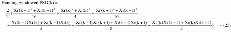
This equation shows why the width of the peak when we applied Hanning window becomes 3 bins when data length is A (Please see Figure 2-6, Figure 4-6(a) or Figure 4-10(c)). Signal at k_th bin affects PSD of k-1, k and k+1_th bins. Although we usually do not call this widening of signal spectral leakage, the basic principles of this widening and spectral leakage are the same as we will describe in Appendix 2. Another important aspect of equation (23) is that it is no longer a simple 3-point weighted moving average unlike equation (22) and we will describe about this topic next. If we use other window functions, we generally do not get such a simple equation as above because Fourier transform of a window function (equation (20)) generally produces many non-zero Wr(n) and Wi(n).

(4-2-7) Implicit FD'Smoothing' Really?
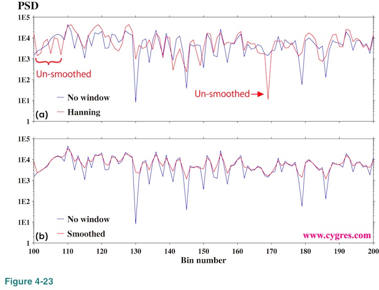
Conclusion first. Applying a window function quite often smoothes resultant PSD but it may un-smoothes in certain cases. Let us show this nature by using Hanning window again. If the right hand side of equation (23) has only the upper part (blue underline), Hanning window will always smooth PSD because equation (19) shows that it becomes a simple 3-point weighted moving average of non-windowed PSD. However, adding the lower part of the right hand side of equation (23) (red underline) makes things complicated because none of the terms in that part is directly related to the non-windowed PSD. Figure 4-23(a) shows part of Hanning windowed PSD (red) and non-windowed PSD (blue) as an example. This graph shows Hanning window smoothed PSD most of the part but there are some exceptions. The red line of Figure 4-23(b) is the result when we use only the upper part of the right hand side of equation (23) (blue underline). This is a simple 3-point weighted moving average of non-widowed PSD (blue) and it always smoothes PSD. If we use Welch's method, lower part of the right hand side of equation (23) will be related to the cross correlation among Xr(k-1), Xr(k), Xr(k+1), Xi(k-1), Xi(k) and Xi(k+1). Based on common statistical theory applied to PSD, we can expect that these terms are un-correlated each other. Thus, lower part of the right hand side of equation (23), will become small as we average over many sets of PSD. Therefore, Welch's method generally provides extra smoothing.

(4-2-8) Reduction of PSD and amplitude due to the window
Application of a window function reduces values of both PSD and amplitude spectrum. This is simply due to the reduction of amplitude of data we feed to PSD computation as we can see in Figure 4-15 and Figure 4-17. To correct this reduction we apply relatively commonly used method. Namely, we compute following values, CP and CA

We multiply PSD by CP and amplitude spectrum by CA to correct reduction. The important point about this correction is that this method only uses information about a window function.

(4-2-9) Does correction of reduction of PSD work well?
Let's look at amplitude spectrum first. The criterion we can use to judge how well the correction of reduction due to windowing is done is the closeness of the corrected signal amplitude to the actual signal amplitude. Judging from Figure 2-7(a), Figure 2-7(b), Figure 2-7(c), Figure 2-13(c), Figure 2-13(e) and Figure 2-16 among others, we can see that amplitude is corrected well. However, there is a caveat. When we applied Hanning window, amplitudes of bins next to the signal bin is 1/2 of the amplitude of the signal bin when frequency match is achieved as we showed in Figure 2-7(a). However, the actual amplitudes of these bins are zero. This difference is caused by implicit FDS of a Hanning window function and the correction we described above would not correct this type of discrepancy.

In case of PSD, it is slightly more complicated because we can think of two criteria to judge the performance of correction. The first one is the same as the one we used for amplitude correction. Another one is that how well equation (1) holds. Since windowing reduces magnitude of data, magnitude of resultant PSD is also reduced. Therefore, without correction the right hand side of equation (1) becomes smaller than the left hand side of equation (1). Here we assume that the "data" in the left hand side of equation (1) is not windowed data but the original one since we usually are not interested in variance of windowed (thus reduced) data. Equation (1) is very important for PSD.

Figure 4-24(a) shows how PSD of the bin where signal exist (we called it signal bin before) varies as we add more data when data contains only a single frequency sinusoid but nothing else. The data we used here is exactly the same as the one shown in Figure 2-4(a). We computed PSD without detrending to avoid effect of artificial inclination we described in (4-1-3) and the reduction of PSD due to the window is corrected using the method described above. The reason why PSD increases as we add more data is that the frequency bandwidth of the bin decreases as we add more data (Figure 2-4(f)) while signal amplitude itself does not change. We show this graph only to demonstrate that PSD increases as we add more data even if we keep everything else the same but there is nothing wrong about it.

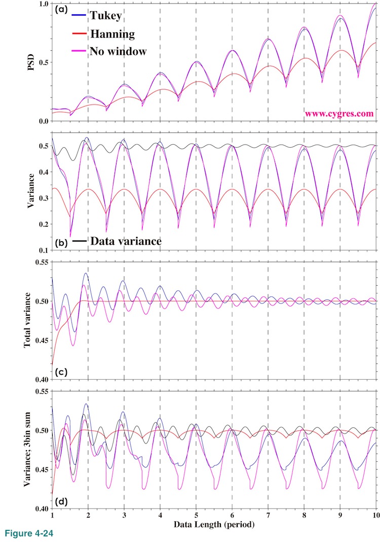
Since graph like Figure 4-24(a) is not convenient to interpret results, we computed variance of the signal bin by multiplying PSD of the signal bin by the frequency bandwidth. Let us call this value, signal bin variance. Figure 4-24(b) shows signal bin variance when we applied Tukey window (blue), Hanning window (red) and when we did not apply any window (purple). The black solid line is the variance of data and this value becomes 0.5 when data length is such that the data is terminated exactly at the end of the cycle of the signal (frequency match; vertical black dashed line). This graph shows that the Hanning windowed signal bin variance is consistently smaller than others. This might make us conclude that the correction of reduction is wrong based on the first criterion.

Now let us use the second criterion. As we described before, Hanning window makes width of peak of PSD wider. Figure 4-24(c) shows the results of summation of variance of all of the bins except zero frequency bin (left hand side of equation (1)). The result of non-windowed PSD (purple) in this graph becomes the same as data variance (black line in Figure 4-24(b)) by equation (1) and, thus, we did not draw data variance. This graph shows that the summed variance of Hanning windowed PSD is not particularly smaller than other cases. Figure 4-24(d) shows results of summation of variance of 3 consecutive bins, center of which is the signal bin. This graph shows that 3-bin summation of variance of Hanning windowed PSD is much closer to the variance of data and its variation is much smaller. If we look at this graph carefully we can see that the 3-bin summation of variance of Hanning windowed PSD and data variance both becomes 0.5 where frequency match occurs (vertical black dashed line). Therefore, we can say that the correction of reduction of PSD is done well based on the second criterion.

This apparent contradiction of the results of these two criteria comes from the fact that implicit FDS of window functions would modify frequency resolution of resultant PSD. In other word, we have to use larger frequency bandwidth to compute signal bin variance in Figure 4-24(b). We describe more about this issue in (4-3-3). Our conclusion here is that the correction applied to PSD works well but we need to consider the actual frequency resolution when we use a value of PSD.

We applied these corrections to all of the examples we have shown in this document. As these graphs show, correction generally works well both for PSD and amplitude spectrum. However if characteristic of data varies a lot from one moment to another as in the case of Figure 4-17, this method might not work well for specific frequency ranges.

(4-2-10) Tukey window; how taper ratio affects its characteristics
Conclusion first. Smaller taper ratio gives higher frequency resolution and larger taper ratio gives more accurate PSD and amplitude spectrum. If data is similar to the one described in (4-2-3), we would have a similar problem if we use larger taper ratio.

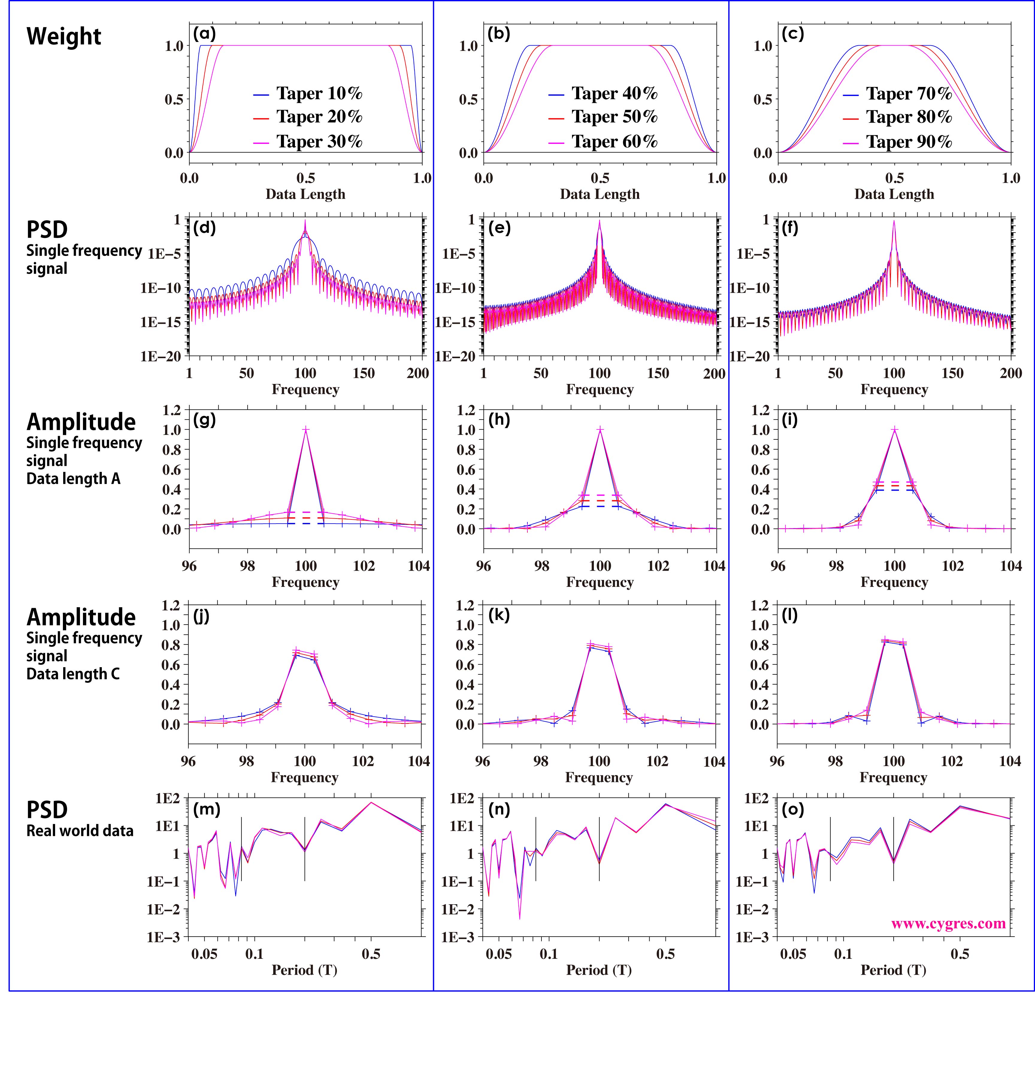
Figure 4-25 shows a value (weight) of 50% tapered Tukey window function as an example. If we applied this window to the data, the first 25% and the last 25% of data will be tapered (reduced) but 50% of the data in the middle will be unaffected (weight equals 1.0). The characteristic of Tukey window varies from the one equivalent to that of non-window by setting taper ratio to 0% to the one equivalent to that of Hanning window by setting taper ratio to 100% as we mentioned before.

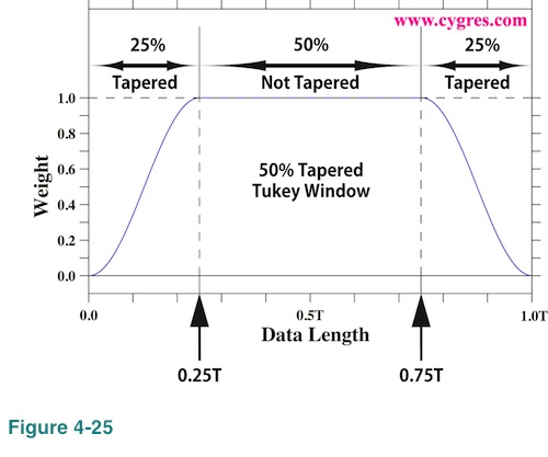
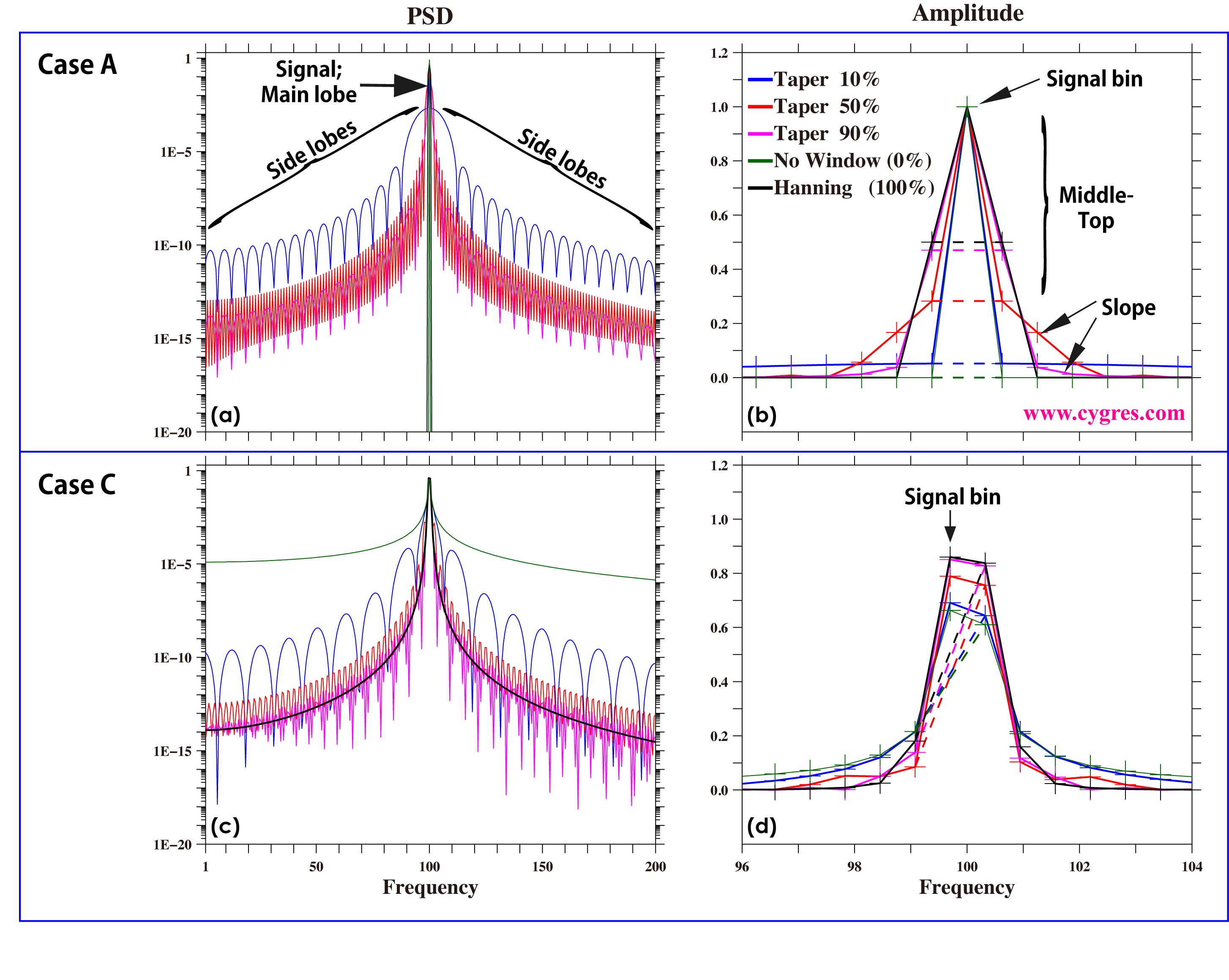
Figure 4-26(a) shows part of PSD when we applied 10% tapered (blue), 50% tapered (red) and 90% tapered (purple) Tukey window as well as part of PSD when we did not apply any window (dark green; equivalent to 0% tapered Tukey window) and when we applied Hanning window (black; equivalent to 100% tapered Tukey window). The data we used for these computations contains only a single sinusoid, frequency of which is 100. This data is the same as the one shown in Figure 2-4(a) except for frequency. The data length is adjusted so that the frequency match is achieved (data length A in Figure 2-4(a)). In this case, non-windowed PSD (dark green) shows that only one bin, frequency of which is exactly the same as signal frequency, contains entire variations of data and PSDs of all other bins are zero within computational accuracy (blue line in Figure 4-5(a)). In other words, there is no spectral leakage and this is true even if we applied any window function. However, this graph shows Tukey windowed PSDs have many bumps labeled side lobes. The reason why they exist is that the Fourier transform of Tukey window produces many non-zero Wr(n)s and Wi(n)s in equation (20) unlike Hanning window, and those non-zero coefficients spread the effect of the signal to an entire frequency range. As we will describe in Appendix 2, cause of this side lobes is practically the same as the cause of spectral leakage. The magnitudes of side lobes are symmetrical with respect to the signal bin and they decrease as taper ratio increases. As we mentioned before, we will see side lobes even in the case when we applied Hanning window if we compute continuous PSD (Appendix 2).

Figure 4-26(b) shows an expanded view of amplitude spectra near the signal bin. This part is often called a main lobe. We drew dashed lines connecting bins adjacent to the signal bin to show how the 'local' width of peak varies. This graph shows that the values of the bins next to the signal bin steadily increase (dashed lines shift upward) and top to middle part of 'mountain' becomes wider as taper ratio increases. However, if we look at the width of the 'slope' part of this 'mountain', 50% tapered Tukey window gives us the widest 'slope' in this graph. Figure 4-26(a) shows that overall, or global, sharpness of the peak increases if we use a larger taper ratio but Figure 4-26(b) shows that 'local' sharpness decresases if we only look at few bins near the signal bin.

Figure 4-26(c) shows the same as Figure 4-26(a) does except that we have changed the data length so that the difference between frequency of the signal bin and the actual signal frequency becomes the largest (data length C in Figure 2-4(a)). In this case we expect large spectral leakage occurs. Non-windowed PSD (dark green) shows the largest PSD across the entire frequency range and this is caused by spectral leakage. Tukey windowed PSDs in this graph are not that much different from those in Figure 4-26(a) in term of amplitude although the shapes of side lobes are different. Hanning windowed PSD does not have bumps but the magnitude is close to the 90% tapered Tukey windowed PSD as we expected. Figure 4-26(d) shows the same as Figure 4-26(b) does except for the data length. Amplitude of signal bin approaches closer to the actual signal amplitude (1.0) as taper ratio increases but the amplitude of a bin to the left of the signal bin also increases and the top of the 'mountain' becomes flatter. Variations of amplitudes at 'slope' are somewhat complicated as before.

In short, Figure 4-26 shows that smaller taper ratio gives us higher frequency resolution (sharper main lobe) but larger taper ratio gives us better PSD (closer to actual PSD).

Figure 4-27(a) shows PSD of real data when we applied 10% tapered (blue), 50% tapered (red) and 90% tapered (purple) Tukey window as well as PSD when we did not apply any window (dark green) and when we applied Hanning window (black). The time series of this data is shown in Figure 4-15(a). Since this graph is too complicated to make comparisons, we applied a 3-bin FDS and the results are shown in Figure 4-27(b). The differences among PSDs are most prominent within Band B as expected because large variations within band B are concentrated near both ends of data (Figure 4-17). However, in general, we feel differences are relatively small for casual use of PSD. These graphs suggest that, although the side lobes of Tukey window in Figure 4-26 are annoying, their actual effects may be negligible for majority of practical applications.

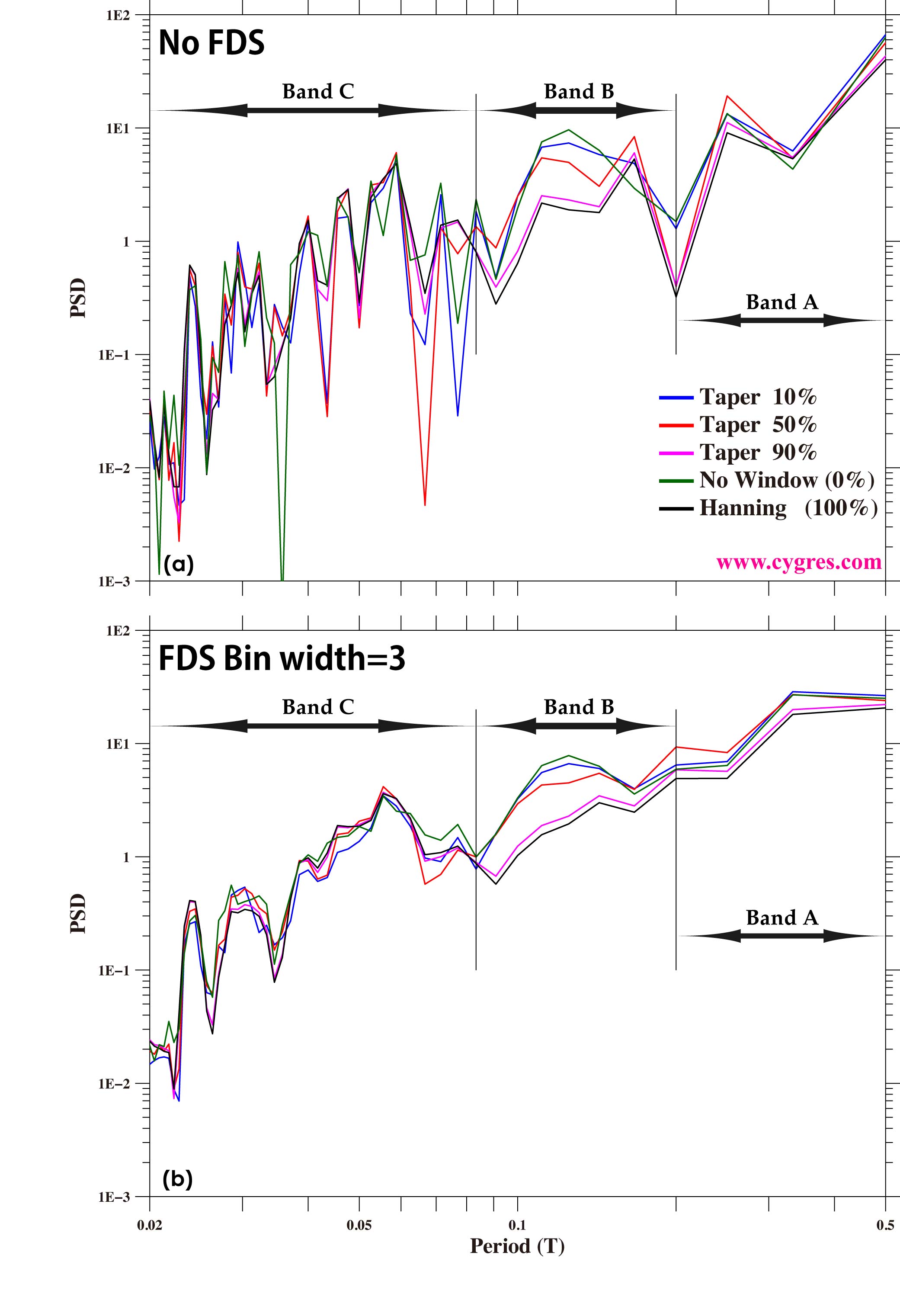
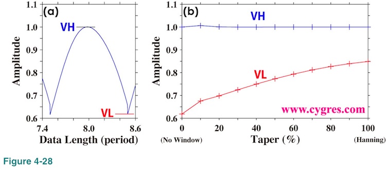
Figure 4-28(b) shows how the maximum and the minimum amplitudes change as taper ratio increases. Here the maximum amplitude is the amplitude when the frequency of the signal bin matches actual signal frequency (VH in Figure 4-28(a)) and the minimum amplitude is the amplitude when difference between frequency of the signal bin and actual signal frequency becomes the largest (VL in Figure 4-28(a)). As we mentioned before, Tukey window becomes Hanning window when taper ratio is 100%. When we deal with real world data, it is usually difficult to achieve frequency matches. Therefore, it would be better if the difference between VH and VL were small. This graph shows that larger taper ratio gives smaller difference between VH and VL. Thus, again, larger taper ratio would likely give us more accurate PSD.

Finally we show how PSD and amplitude vary when we change taper ratio from 10% to 90% with 10% increment in Figure 4-29. The first row ((a), (b) and (c)) shows the shapes of Tukey window. The second row ((d), (e) and (f)) shows PSDs similar to the one shown in Figure 4-26(a). The third row ((g), (h) and (i)) shows amplitude spectra similar to the one shown in Figure 4-26(b). The fourth row ((j), (k) and (l)) shows amplitude spectra similar to the one shown in Figure 4-26(d). The fifth row ((m), (n) and (o)) shows PSDs similar to the one shown in Figure 4-27(a). We grouped results of three different taper ratios together. The taper ratios and corresponding color codes are shown in the first row for each column. We hope this document will provide enough information so that our customers can determine proper taper ratio.

To read next page, please click right button below.